NLP Lecture: Bigram Frequencies and Smoothing Techniques

1. Natural Language Processing Lecture 7—2/3/2015 Susan W. Brown

2. Today • Problem set 1 • Last bit of n-grams • Programming assignment 1 • Parts of Speech

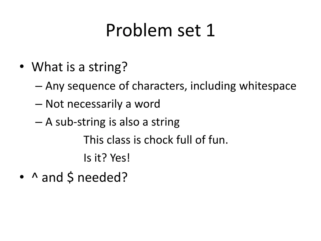
3. Problem set 1 • What is a string? – Any sequence of characters, including whitespace – Not necessarily a word – A sub-string is also a string This class is chock full of fun. Is it? Yes! • ^ and $ needed?

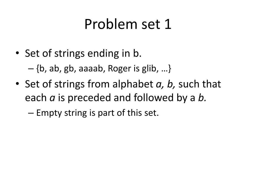
4. Problem set 1 • Set of strings ending in b. – {b, ab, gb, aaaab, Roger is glib, …} • Set of strings from alphabet a, b, such that each a is preceded and followed by a b. – Empty string is part of this set.

5. Back to N-grams • Using probablities of n-grams to predict (or generate) next word • What to do with zero counts?

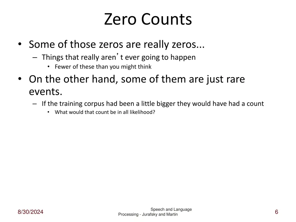
6. Zero Counts • Some of those zeros are really zeros... – Things that really aren’t ever going to happen • Fewer of these than you might think • On the other hand, some of them are just rare events. – If the training corpus had been a little bigger they would have had a count • What would that count be in all likelihood? Speech and Language 8/30/2024 6 Processing - Jurafsky and Martin

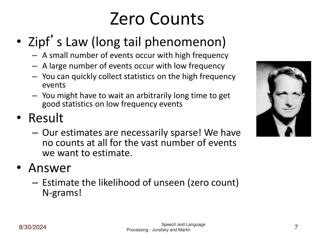
7. Zero Counts • Zipf’s Law (long tail phenomenon) – A small number of events occur with high frequency – A large number of events occur with low frequency – You can quickly collect statistics on the high frequency events – You might have to wait an arbitrarily long time to get good statistics on low frequency events • Result – Our estimates are necessarily sparse! We have no counts at all for the vast number of events we want to estimate. • Answer – Estimate the likelihood of unseen (zero count) N-grams! Speech and Language 8/30/2024 7 Processing - Jurafsky and Martin

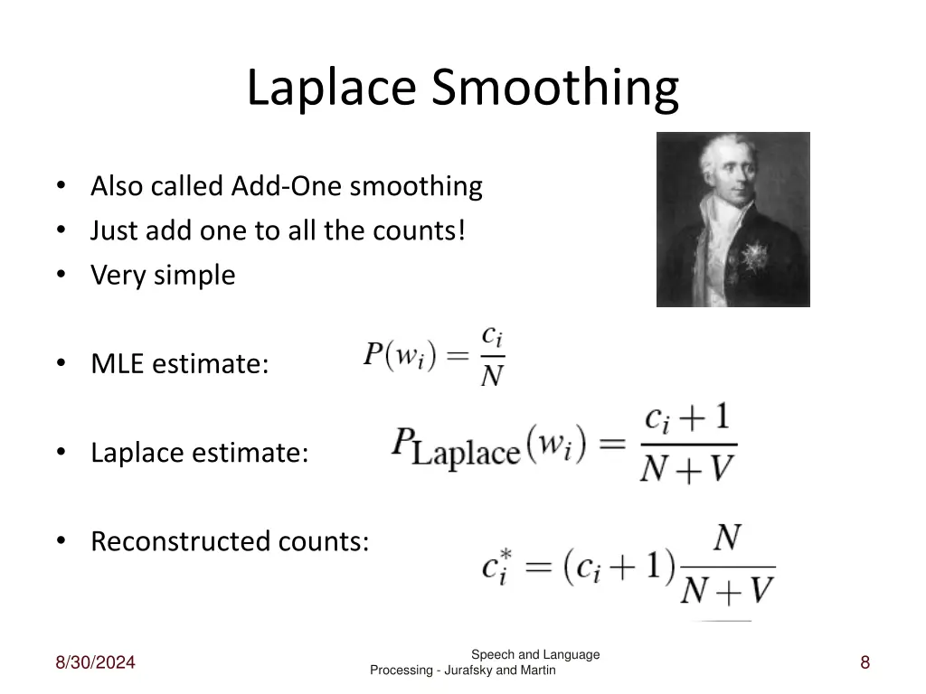
8. Laplace Smoothing • Also called Add-One smoothing • Just add one to all the counts! • Very simple • MLE estimate: • Laplace estimate: • Reconstructed counts: Speech and Language 8/30/2024 8 Processing - Jurafsky and Martin

9. Big Change to the Counts! • • • C(want to) went from 608 to 238! P(to|want) from .66 to .26! Discount d= c*/c – d for “chinese food” =.10!!! A 10x reduction – So in general, Laplace is a blunt instrument – Could use more fine-grained method (add-k) But Laplace smoothing not generally used for N-grams, as we have much better methods Despite its flaws Laplace (add-k) is however still used to smooth other probabilistic models in NLP, especially – For pilot studies – In document classification – Information retrieval – In domains where the number of zeros isn’t so huge. • • Speech and Language 8/30/2024 9 Processing - Jurafsky and Martin

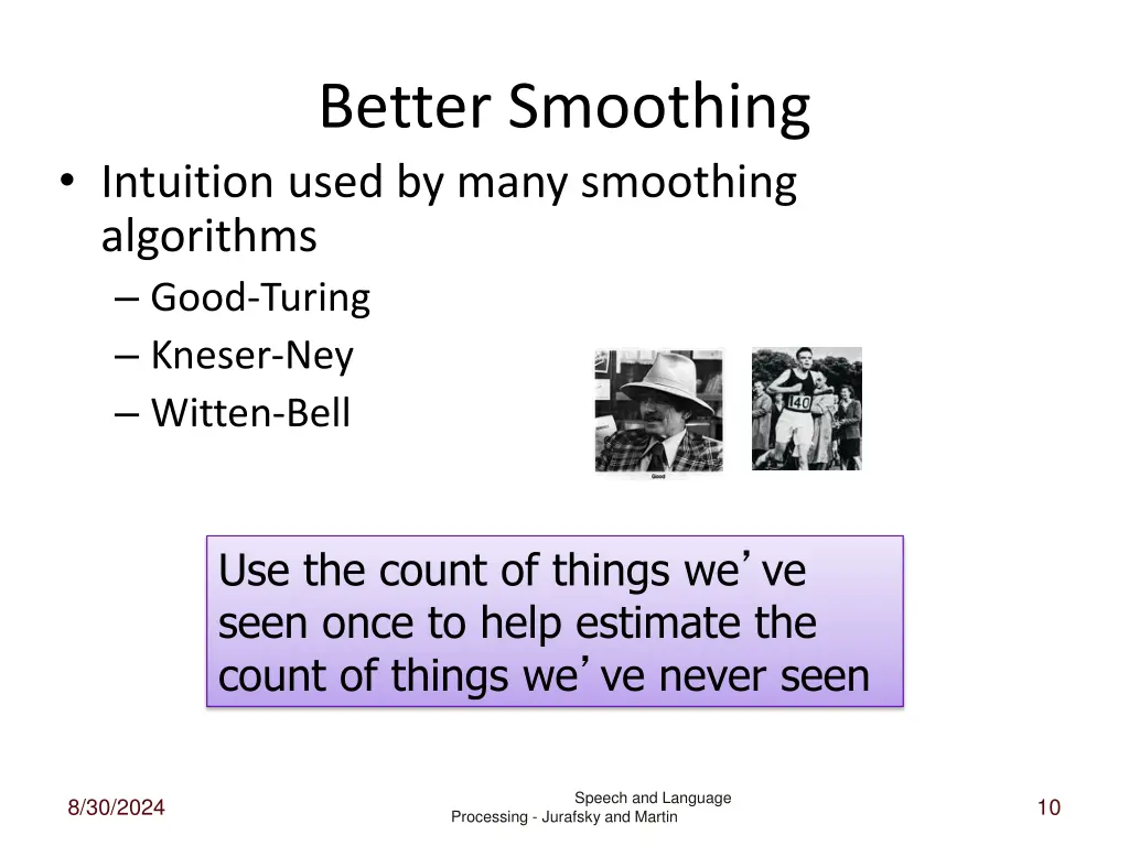
10. Better Smoothing • Intuition used by many smoothing algorithms – Good-Turing – Kneser-Ney – Witten-Bell Use the count of things we’ve seen once to help estimate the count of things we’ve never seen Speech and Language 8/30/2024 10 Processing - Jurafsky and Martin

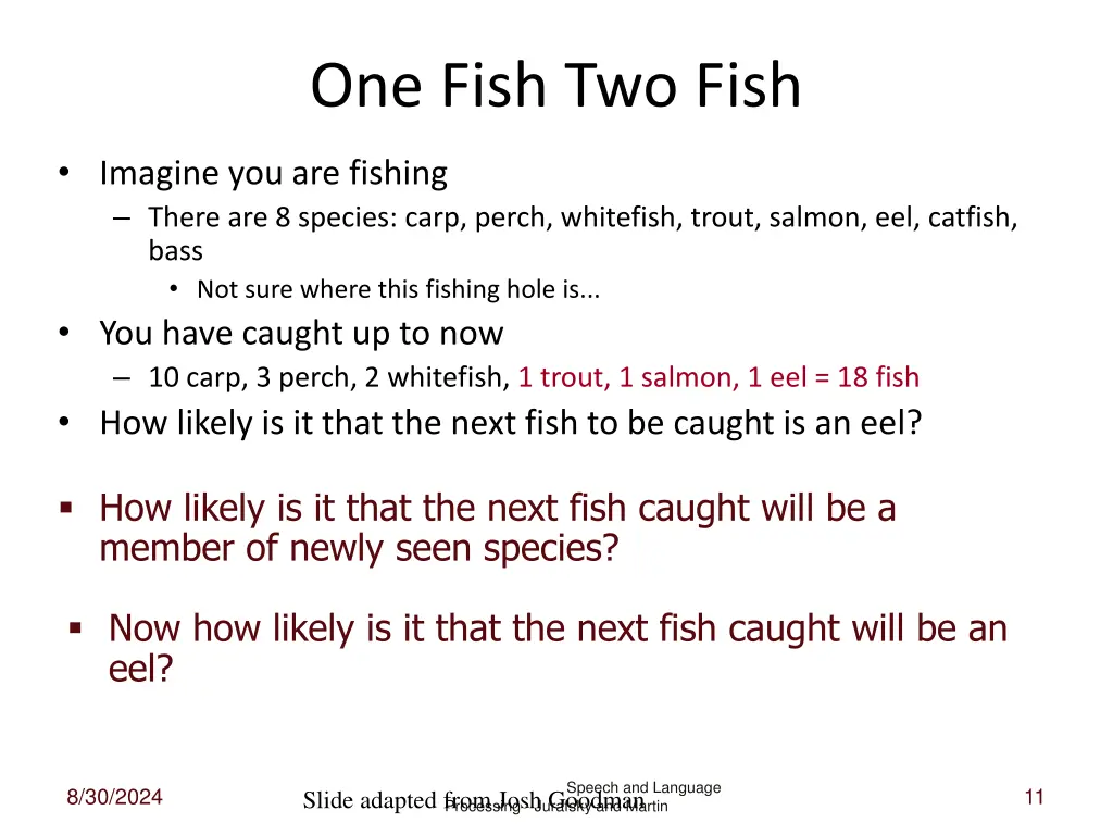
11. One Fish Two Fish • Imagine you are fishing – There are 8 species: carp, perch, whitefish, trout, salmon, eel, catfish, bass • Not sure where this fishing hole is... • You have caught up to now – 10 carp, 3 perch, 2 whitefish, 1 trout, 1 salmon, 1 eel = 18 fish • How likely is it that the next fish to be caught is an eel?  How likely is it that the next fish caught will be a member of newly seen species?  Now how likely is it that the next fish caught will be an eel? Speech and Language 8/30/2024 11 Slide adapted from Josh Goodman Processing - Jurafsky and Martin

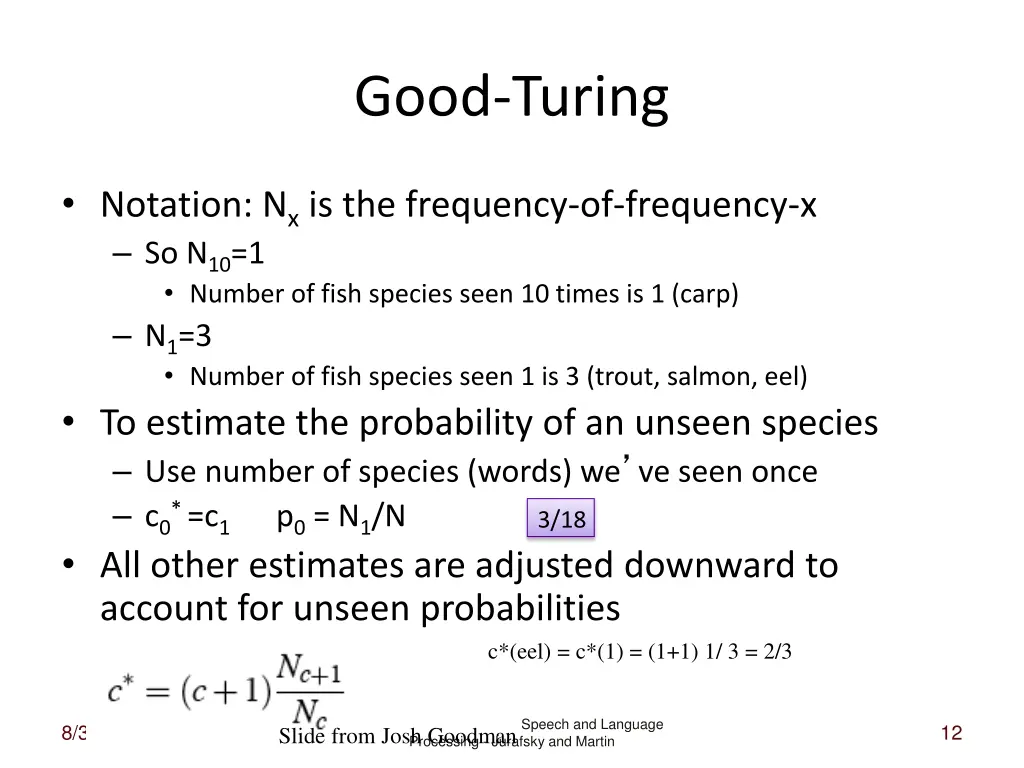
12. Good-Turing • Notation: Nxis the frequency-of-frequency-x – So N10=1 • Number of fish species seen 10 times is 1 (carp) – N1=3 • Number of fish species seen 1 is 3 (trout, salmon, eel) • To estimate the probability of an unseen species – Use number of species (words) we’ve seen once – c0* =c1 p0= N1/N • All other estimates are adjusted downward to account for unseen probabilities 3/18 c*(eel) = c*(1) = (1+1) 1/ 3 = 2/3 Speech and Language 8/30/2024 12 Slide from Josh Goodman Processing - Jurafsky and Martin

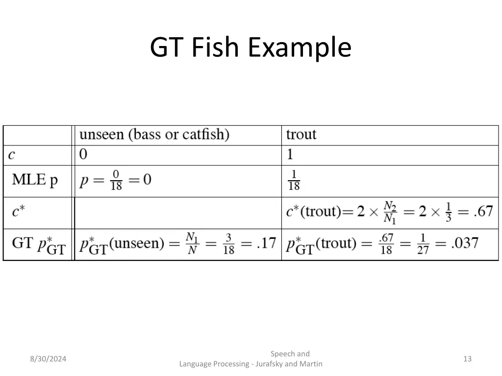
13. GT Fish Example Speech and 8/30/2024 13 Language Processing - Jurafsky and Martin

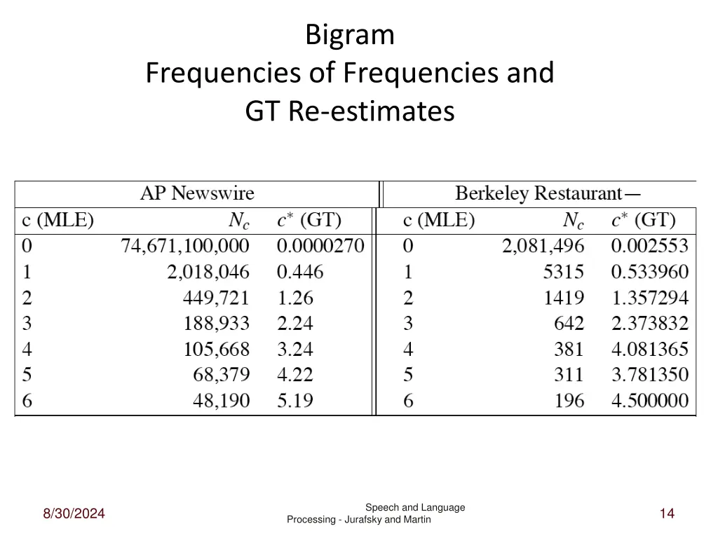
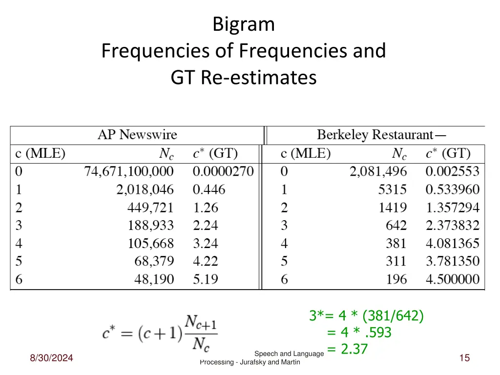
14. Bigram Frequencies of Frequencies and GT Re-estimates Speech and Language 8/30/2024 14 Processing - Jurafsky and Martin

15. Bigram Frequencies of Frequencies and GT Re-estimates 3*= 4 * (381/642) = 4 * .593 = 2.37 Speech and Language 8/30/2024 15 Processing - Jurafsky and Martin

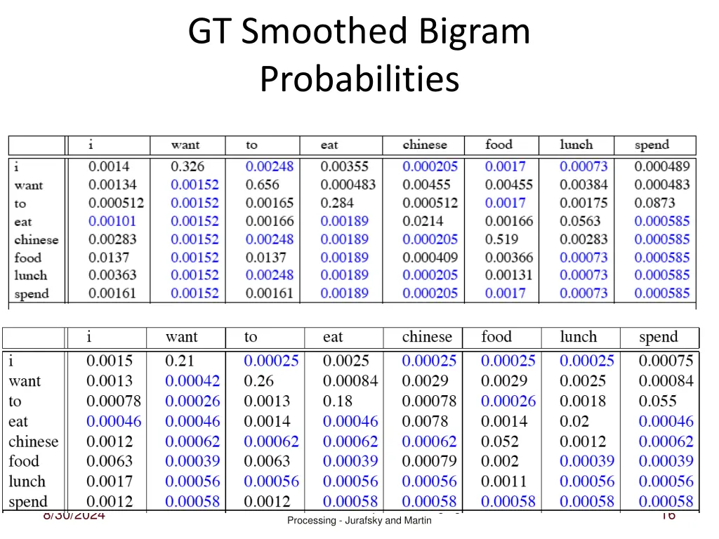
16. GT Smoothed Bigram Probabilities Speech and Language 8/30/2024 16 Processing - Jurafsky and Martin

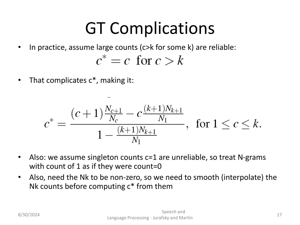
17. GT Complications • In practice, assume large counts (c>k for some k) are reliable: • That complicates c*, making it: • Also: we assume singleton counts c=1 are unreliable, so treat N-grams with count of 1 as if they were count=0 Also, need the Nk to be non-zero, so we need to smooth (interpolate) the Nk counts before computing c* from them • Speech and 8/30/2024 17 Language Processing - Jurafsky and Martin

18. More zero counts • What if a frequency of frequency count is zero? • Remember Zipf’s law • Linear regression mapping Nc to c in log space

19. Toolkits • With FSAs/FSTs... – Openfst.org • For language modeling – SRILM • SRI Language Modeling Toolkit • All the bells and whistles you can imagine Speech and Language 8/30/2024 19 Processing - Jurafsky and Martin

20. End of chapter 4 • Not covering 4.9 in lecture; read it for the problems presented and the intuition of the solutions • 4.10 and 4.11 will not come up in the exam

21. Programming assignment 1 • Due Thursday, Feb. 5, midnight • Import re • What is a word? • What is the context of the end and beginning of a sentence? • What is different between this and abbreviations? • Perfect counts not the ultimate test of a good script. Generalize. Do not over-fit your example.

22. Back to Some Linguistics Speech and Language 8/30/2024 22 Processing - Jurafsky and Martin

23. Word Classes: Parts of Speech • 8 (ish) traditional parts of speech – Noun, verb, adjective, preposition, adverb, article, interjection, pronoun, conjunction, etc. – Also known as • parts-of-speech, lexical categories, word classes, morphological classes, lexical tags... – Lots of debate within linguistics and cognitive science community about the number, nature, and universality of these • We’ll completely ignore this debate Speech and Language 8/30/2024 23 Processing - Jurafsky and Martin

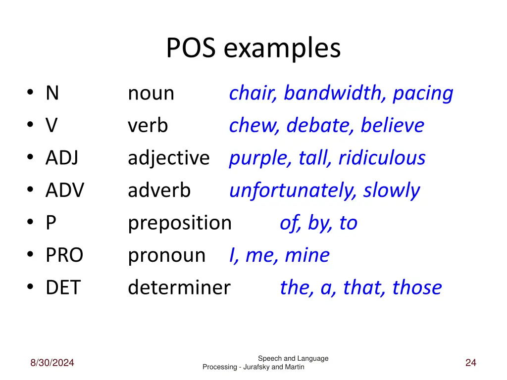
24. POS examples • N • V • ADJ • ADV • P • PRO • DET noun verb adjective purple, tall, ridiculous adverb unfortunately, slowly preposition pronoun I, me, mine determiner chair, bandwidth, pacing chew, debate, believe of, by, to the, a, that, those Speech and Language 8/30/2024 24 Processing - Jurafsky and Martin

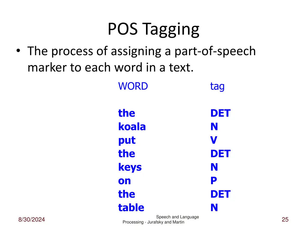
25. POS Tagging • The process of assigning a part-of-speech marker to each word in a text. WORD tag the koala put the keys on the table DET N V DET N P DET N Speech and Language 8/30/2024 25 Processing - Jurafsky and Martin

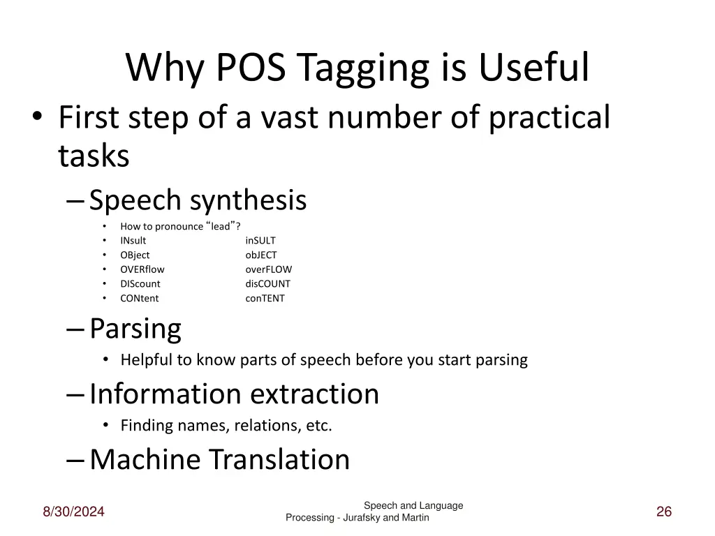
26. Why POS Tagging is Useful • First step of a vast number of practical tasks –Speech synthesis • How to pronounce “lead”? • INsult inSULT • OBject obJECT • OVERflow overFLOW • DIScount disCOUNT • CONtent conTENT –Parsing • Helpful to know parts of speech before you start parsing –Information extraction • Finding names, relations, etc. –Machine Translation Speech and Language 8/30/2024 26 Processing - Jurafsky and Martin

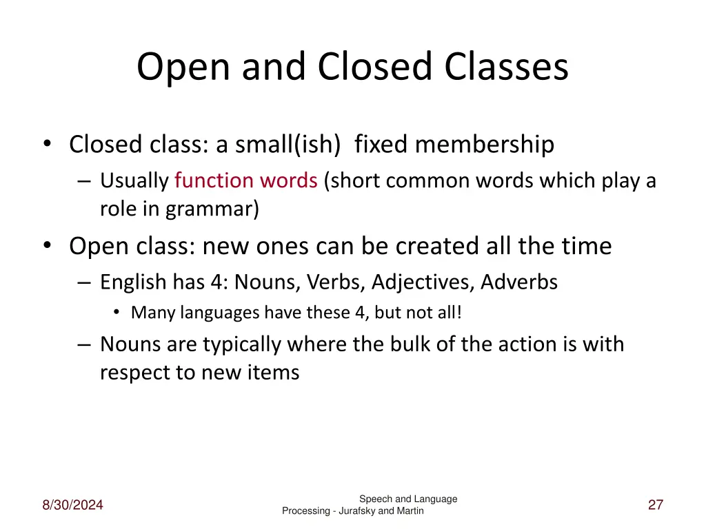
27. Open and Closed Classes • Closed class: a small(ish) fixed membership – Usually function words (short common words which play a role in grammar) • Open class: new ones can be created all the time – English has 4: Nouns, Verbs, Adjectives, Adverbs • Many languages have these 4, but not all! – Nouns are typically where the bulk of the action is with respect to new items Speech and Language 8/30/2024 27 Processing - Jurafsky and Martin

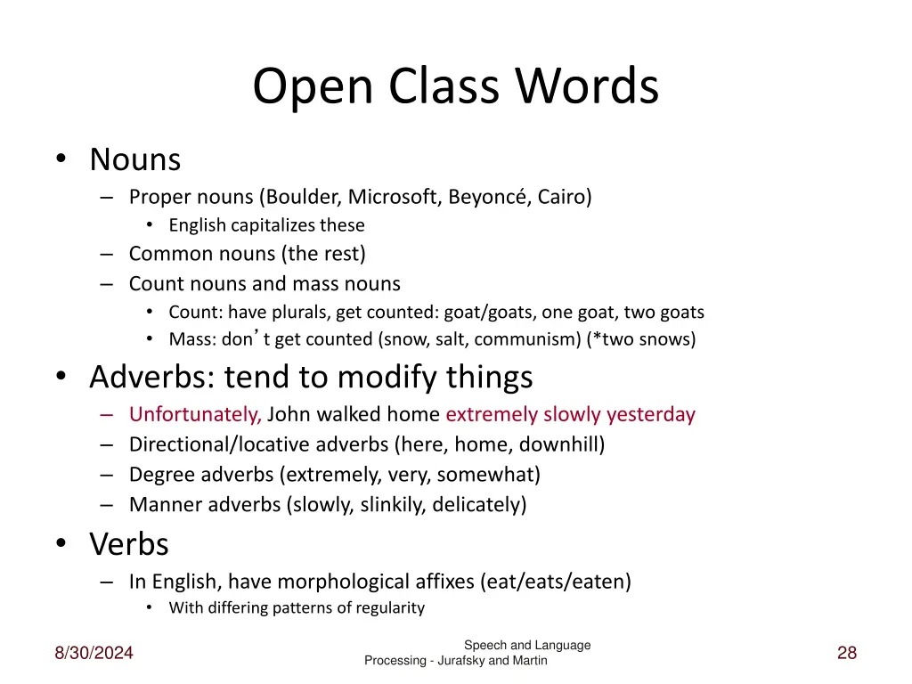
28. Open Class Words • Nouns – Proper nouns (Boulder, Microsoft, Beyoncé, Cairo) • English capitalizes these – Common nouns (the rest) – Count nouns and mass nouns • Count: have plurals, get counted: goat/goats, one goat, two goats • Mass: don’t get counted (snow, salt, communism) (*two snows) • Adverbs: tend to modify things – Unfortunately, John walked home extremely slowly yesterday – Directional/locative adverbs (here, home, downhill) – Degree adverbs (extremely, very, somewhat) – Manner adverbs (slowly, slinkily, delicately) • Verbs – In English, have morphological affixes (eat/eats/eaten) • With differing patterns of regularity Speech and Language 8/30/2024 28 Processing - Jurafsky and Martin

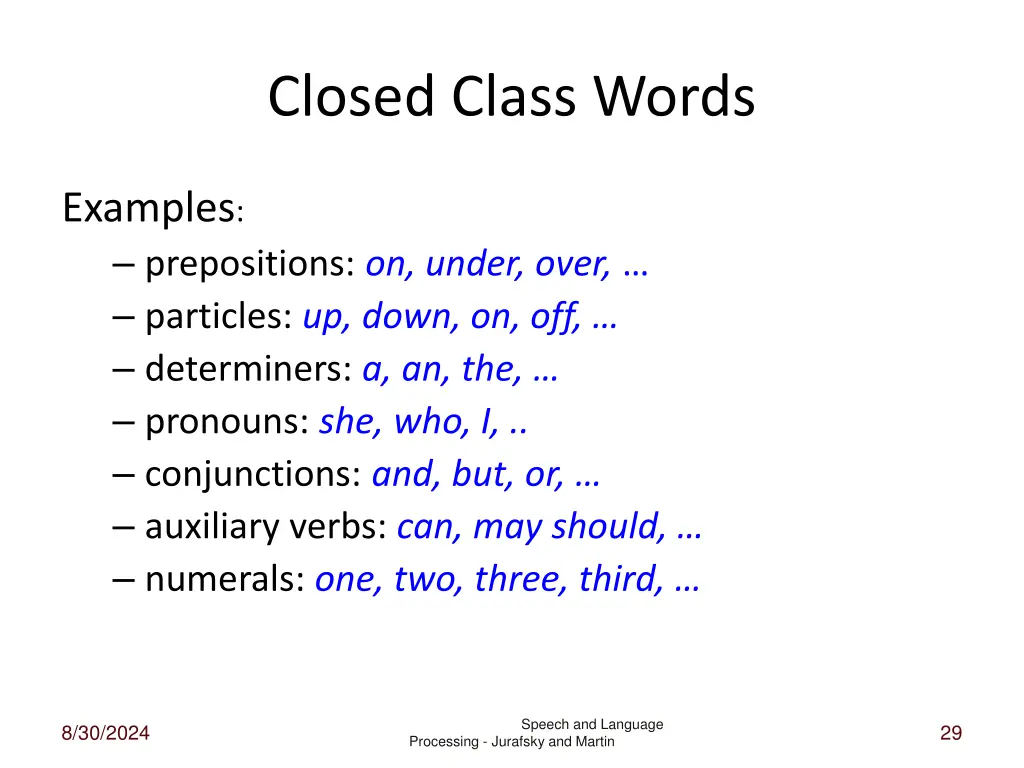
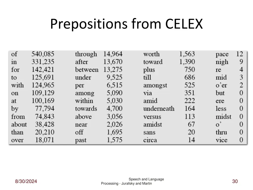
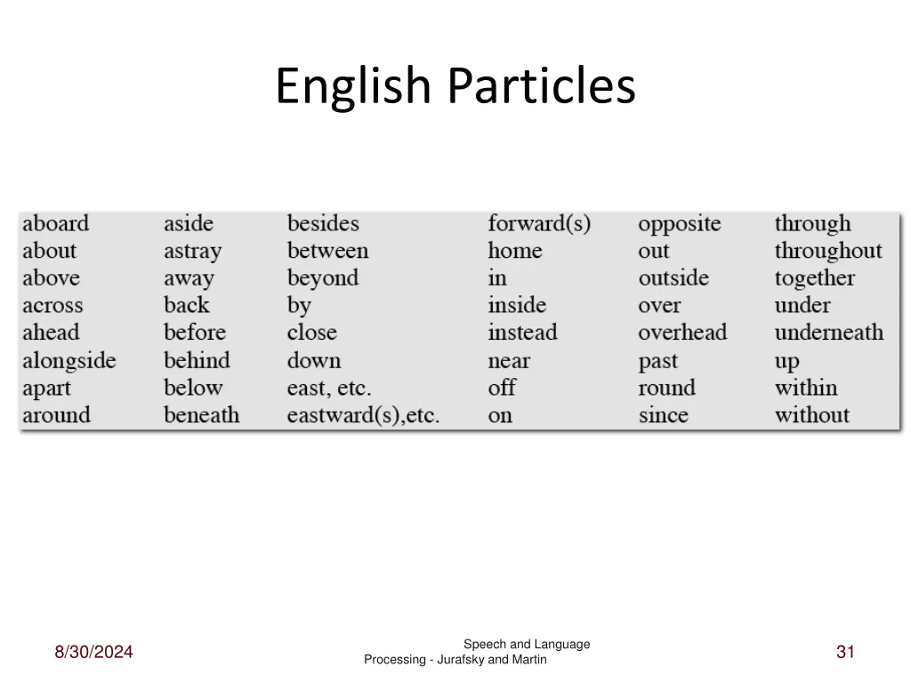
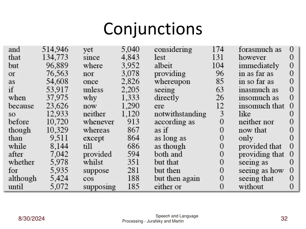
29. Closed Class Words Examples: – prepositions: on, under, over, … – particles: up, down, on, off, … – determiners: a, an, the, … – pronouns: she, who, I, .. – conjunctions: and, but, or, … – auxiliary verbs: can, may should, … – numerals: one, two, three, third, … Speech and Language 8/30/2024 29 Processing - Jurafsky and Martin

30. Prepositions from CELEX Speech and Language 8/30/2024 30 Processing - Jurafsky and Martin

31. English Particles Speech and Language 8/30/2024 31 Processing - Jurafsky and Martin

32. Conjunctions Speech and Language 8/30/2024 32 Processing - Jurafsky and Martin

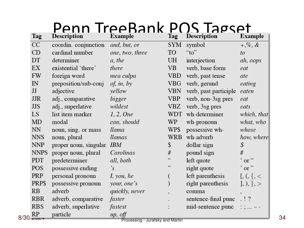
33. POS Tagging: Choosing a Tagset • There are many potential distinctions we can draw leading to potentially large tagsets • To do POS tagging, we need to choose a standard set of tags to work with • Could pick very coarse tagsets – N, V, Adj, Adv. • More commonly used set is the finer grained, “Penn TreeBank tagset”, 45 tags – PRP$, WRB, WP$, VBG • Even more fine-grained tagsets exist Speech and Language 8/30/2024 33 Processing - Jurafsky and Martin

34. Penn TreeBank POS Tagset Speech and Language 8/30/2024 34 Processing - Jurafsky and Martin

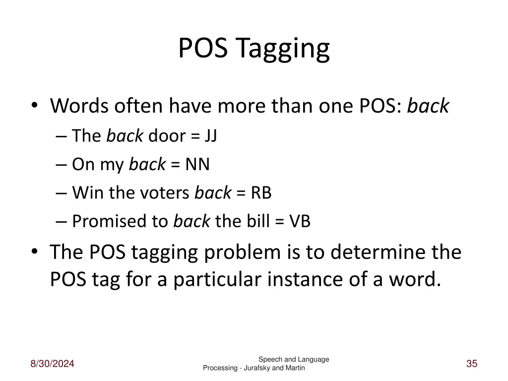
35. POS Tagging • Words often have more than one POS: back – The back door = JJ – On my back = NN – Win the voters back = RB – Promised to back the bill = VB • The POS tagging problem is to determine the POS tag for a particular instance of a word. Speech and Language 8/30/2024 35 Processing - Jurafsky and Martin

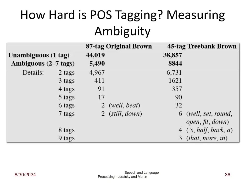
36. How Hard is POS Tagging? Measuring Ambiguity Speech and Language 8/30/2024 36 Processing - Jurafsky and Martin

37. Two Methods for POS Tagging 1. Rule-based tagging – See the text 2. Stochastic 1. Probabilistic sequence models • HMM (Hidden Markov Model) tagging • MEMMs (Maximum Entropy Markov Models) Speech and Language 8/30/2024 37 Processing - Jurafsky and Martin

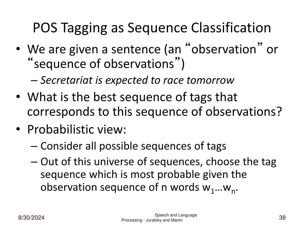
38. POS Tagging as Sequence Classification • We are given a sentence (an “observation” or “sequence of observations”) – Secretariat is expected to race tomorrow • What is the best sequence of tags that corresponds to this sequence of observations? • Probabilistic view: – Consider all possible sequences of tags – Out of this universe of sequences, choose the tag sequence which is most probable given the observation sequence of n words w1…wn. Speech and Language 8/30/2024 38 Processing - Jurafsky and Martin

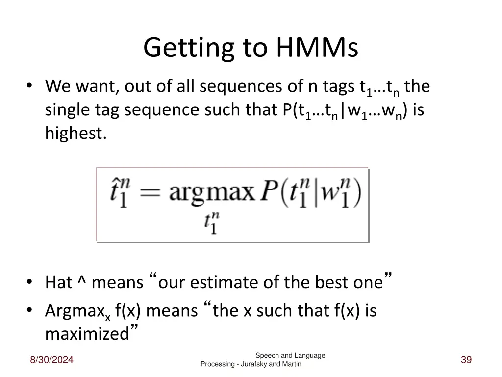
39. Getting to HMMs • We want, out of all sequences of n tags t1…tnthe single tag sequence such that P(t1…tn|w1…wn) is highest. • Hat ^ means “our estimate of the best one” • Argmaxxf(x) means “the x such that f(x) is maximized” Speech and Language 8/30/2024 39 Processing - Jurafsky and Martin

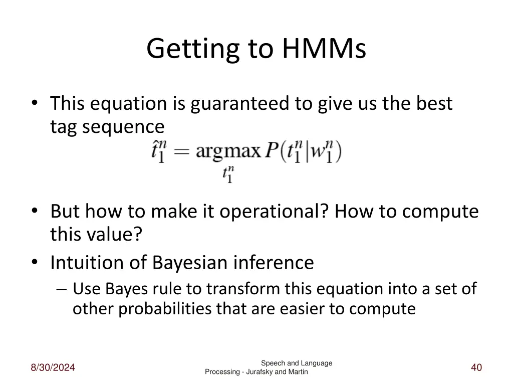
40. Getting to HMMs • This equation is guaranteed to give us the best tag sequence • But how to make it operational? How to compute this value? • Intuition of Bayesian inference – Use Bayes rule to transform this equation into a set of other probabilities that are easier to compute Speech and Language 8/30/2024 40 Processing - Jurafsky and Martin

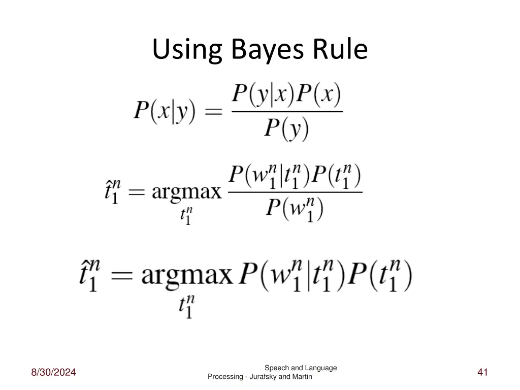
41. Using Bayes Rule Speech and Language 8/30/2024 41 Processing - Jurafsky and Martin

42. Thursday • More POS tagging • Bayesian inference • Finish chapter 5