Numerical Relativity: Generalized Harmonic Coordinates
320 likes | 343 Views
Learn about black hole simulations using harmonic coordinates, constraint damping, and results from close binary mergers. Discover a brief overview of numerical relativity with AMR and coordinate compactification for stable evolution.

Numerical Relativity: Generalized Harmonic Coordinates
E N D
Presentation Transcript
Binary Black Hole Simulations Frans Pretorius University of Alberta Numerical Relativity2005: Compact BinariesNov 2-4, 2005 NASA’s Goddard Space Flight Center
Outline • Methodology • an evolution scheme based on generalized harmonic coordinates • choosing the gauge • constraint damping • Results • merger of a close binary • an early look at not-so-close binaries • evolution of a Cook-Pfeiffer quasi-circular initial data set • Summary • near future work
Numerical relativity using generalized harmonic coordinates – a brief overview • Formalism • the Einstein equations are re-expressed in terms of generalized harmonic coordinates • add source functions to the definition of harmonic coordinates to be able to choose arbitrary slicing/gauge conditions • add constraint damping terms to aid in the stable evolution of black hole spacetimes • Numerical method • equations discretized using finite difference methods • directly discretize the metric; i.e. no “conjugate variables” introduced • use adaptive mesh refinement (AMR) to adequately resolve all relevant spatial/temporal length scales (still need supercomputers in 3D) • use (dynamical) excision to deal with geometric singularities that occur inside of black holes • add numerical dissipation to eliminate high-frequency instabilities that otherwise tend to occur near black holes • use a coordinate system compactified to spatial infinity to place the physically correct outer boundary conditions
Generalized Harmonic Coordinates • Generalized harmonic coordinates introduce a set of arbitrary source functionsH u into the usual definition of harmonic coordinates • When this condition (specifically its gradient) is substituted for certain terms in the Einstein equations, and the H u are promoted to the status of independent functions, the principle part of the equation for each metric element reduces to a simple wave equation
Generalized Harmonic Coordinates • The claim then is that a solution to the coupled Einstein-harmonic equations which include (arbitrary) evolution equations for the source functions, plus additional matter evolution equations, will also be a solution to the Einstein equations provided the harmonic constraints and their first time derivative are satisfied at the initial time. • “Proof”
An evolution scheme based upon this decomposition • The idea (following Garfinkle[PRD 65, 044029 (2002)]; see also Szilagyi & Winicour[PRD 68, 041501 (2003)]) is to construct an evolution scheme based directly upon the preceding equations • the system of equations is manifestly hyperbolic (if the metric is non-singular and maintains a definite signature) • the hope is that it would be simple to discretize using standard numerical techniques • the ”constraint” equations are the generalized harmonic coordinate conditions • simpler to control “constraint violating modes” when present • one can view the source functions as being analogous to the lapse and shift in an ADM style decomposition, encoding the 4 coordinate degrees of freedom
Coordinate Issues • The source functions encode the coordinate degrees of freedom of the spacetime • how does one specify H u to achieve a particular slicing/spatial gauge? • what class of evolutions equations for H u can be used that will not adversely affect the well posedness of the system of equations?
Specifying the spacetime coordinates • A way to gain insight into how a given H u could affect the coordinates is to appeal to the ADM metric decompositionthenor
Specifying the spacetime coordinates • Therefore, H t (H i ) can be chosen to drivea (b i) to desired values • for example, the following slicing conditions are all designed to keep the lapse from “collapsing”, and have so far proven useful in removing some of the coordinate problems with harmonic time slicing
Constraint Damping • Following a suggestion by C. Gundlach ([C. Gundlach, J. M. Martin-Garcia, G. Calabrese, I. Hinder, gr-qc/0504114] based on earlier work by Brodbeck et al [J. Math. Phys. 40, 909 (1999)]) modify the Einstein equations in harmonic form as follows: where • For positive k, Gundlach et al have shown that all constraint-violations with finite wavelength are damped for linear perturbations around flat spacetime
Effect of constraint damping • Axisymmetric simulation of a Schwarzschild black hole, Painleve-Gullstrand coords. • Left and right simulations use identical parameters except for the use of constraint damping k=0 k=1/(2M)
Merger of a close binary system • initial data – use boosted scalar field collapse to set up the binary • choice for initial geometry: • spatial metric and its first time derivative is conformally flat • maximal (gives initial value of lapse and time derivative of conformal factor) and harmonic (gives initial time derivatives of lapse and shift) • Hamiltonian and Momentum constraints solved for initial values of the conformal factor and shift, respectively • advantages of this approach • “simple” in that initial time slice is singularity free • all non-trivial initial geometry is driven by the scalar field—when the scalar field amplitude is zero we recover Minkowski spacetime • disadvantages • ad-hoc in choice of parameters to produce a desired binary system • uncontrollable amount of “junk” initial radiation (scalar and gravitational) in the spacetime; though all present initial data schemes suffer from this
Merger of a close binary system • Gauge conditions: • Note: this is strictly speaking not spatial harmonic gauge, which is defined in terms of the “vector” components of the source function • Constraint damping term
Orbit • Initially: • equal mass components • eccentricity e ~ 0 - 0.2 • coordinate separation of black holes ~ 13M • proper distance between horizons ~ 16M • velocity of each black hole ~0.16 • spin angular momentum = 0 • ADM Mass ~ 2.4M Simulation (center of mass) coordinates Reduced mass frame; heavier lines are position of BH 1 relative to BH 2 (green star); thinner black lines are reference ellipses • Final black hole: • Mf~ 1.9M • Kerr parameter a ~ 0.70 • error ~ 5%
Lapse function a, orbital plane All animations: time in units of the mass of a single, initial black hole, and from medium resolution simulation
Waveform extraction • Can we extract a waveform in light of • unphysical radiation in initial data • Compactification; i.e. poor resolution near outer boundaries • AMR “noise”: finding the waveform typically requires taking derivatives of metric functions; enhances noise • Answer seems to be yes, though the caveat is how accurately does one need the waveform.
Waveform extraction Real component of the Newman-Penrose scalar Y4timesr,z=0 slice of the solution
Waveform extraction Real component of the Newman-Penrose scalar Y4timesr,x=0 slice of the solution
Waveform extraction Imaginary component of the Newman-Penrose scalar Y4timesr,x=0 slice of the solution
Energy radiated ? • On some sphere of radius R, a large distance from the source: Difficult to integrate accurately from a numerical simulation: • R=25M : 4.7% (% relative to 2M)R=50M : 3.2%R=75M : 2.7% R=100M : 2.3% • Other estimates: • Horizon mass : 5% • From comparison of wave amplitudes from boosted, head-on collision with similar simulation parameters, and known estimates from the literature, also suggests total is around 5%[Hobill et al, PRD 52, 2044 (1995)]; Totals (many caveats!!):
Not-so-close binaries • A couple of questions • the waveform seems to be dominated by the collision/ringdown phase of the orbit. Is this generic? i.e. will the last few cycles of a waveform carry away as much as 5% of the energy of the binary? • need more orbits to be able to make a clearer identification between the orbital vs. merger/ringdown phase of the waveform • how generic is this plunge/ringdown signal to changes in initial conditions? • evolve more initial data
Not-so-close binaries • Initially: • equal mass components • proper distance between horizons ~ 22 M0 • different orbits are from different initial scalar field boost parameters • reference circles of coordinate radius M0and 3.8M0.
Merger of a Cook-Pfeiffer Quasi-Circular Initial Data set • Initial data provided by H. Pfeiffer, based on solutions to the constraint equations with free data and black hole boundary conditions as described in Cook and Pfeiffer, PRD 70, 104016 (2004): • equal mass, corotating black holes • approximate helical killing vector black hole boundary conditions • lapse boundary condition “59a” : d(ay)/dr=0 • free data • conformally flat spatial metric • maximal slice • in the corotating frame, quasi-equilibrium conditions: initial time derivative of conformal metric is 0, and initial time derivative of K=0 • Initial coordinate condition is spacetime harmonic • Coordinate evolution parameters similar to scalar field example before (x=10/ M0 ,z=2/M0 n=6,k=1/M0 ) • Initial binary proper separation for this example is ~ 16 M0, coordinate separation ~ 12 M0.
Orbit • Merges in ~ 1 ½ orbits (though note that resolution still low! … need more simulations to get a better error bar!) • Final Kerr parameter ~ 0.75 • AH mass and Y4 estimates suggest ~5% of the total mass of the system is radiated • Green curve is a scalar field comparison orbit; the one to the left has been scaled so that the masses are equal, the one to the right so that the initial coordinate separation is equal. On the right figure there is also a superimposed a reference circle.
Lapse function a, orbital plane Note: different color scale to earlier lapse animation
Real component of the Newman-Penrose scalar Y4timesr,z=0 slice of the solution Note: different color scale to earlier NP scalar animations
Summary -- near future work • What physics can one hope to extract from these simulations over the next couple of years or so? • very broad initial survey of the qualitative features of the last stages of binary mergers • pick a handful of orbital parameters (mass ratio, eccentricity, initial separation, individual black hole spins) widely separated in parameter space • computational requirements make it completely impractical to try to come up with a template bank for LIGO at this stage (ever?) • try to understand the general features of the emitted waves, the total energy radiated, and range of final spins as a function of the initial parameters, etc.