Download
1 / 66
680 likes | 714 Views
Learn about continuous charge distributions & various charge densities for electric field calculations. Includes examples and principles like Coulomb's Law and Superposition. Also covers Gauss' Law and Electric Flux.

E N D
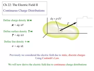
Ch 22: The Electric Field II Continuous Charge Distributions Define charge density r: r = dq/ dV Define surface density s: s = dq/ dA Define line density l: l = dq/ dL Previously we considered the electric field due to static, discrete charges Using Coulomb’s Law. We will now derive the electric field due to continuous charge distributions
22.6 The Electric Field due to a Continuous Charge: When we deal with continuous charge distributions, it is most convenient to express the charge on an object as a charge density rather than as a total charge. For a line of charge, for example, we would report the linear charge density (or charge per unit length) l, whose SI unit is the coulomb per meter. Table 22-2 shows the other charge densities we shall be using.
small piecesof chargedq total chargeQ • Line of charge: dq = ldx l=charge per unit length • Surface of charge: dq = sdA s=charge per unit area • Volume of Charge: • r=charge per unit volume dq = rdV Charge Densities • How do we represent the charge “Q” on an extended object?
How We Calculate (Uniform) Charge Densities: • Examples: • 10 coulombsdistributed over a 2-meter rod. Take total charge, divide by “size” 14 pC(pico = 10-12) distributed over a shell of radius 1 μm. 14 pCdistributed over a sphere of radius 1 mm.
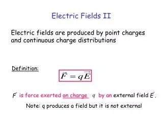
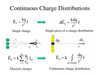
For discrete charges the electric field is a sum For continuous charges, the sum becomes a continuous integral E = S E q Ch 22: The electric field II Continuous Charge Distributions For a small element of charge, dq, the electric field can be obtained from Coulomb’s law for a point charge
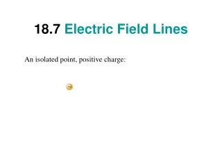
E(r) = ? r ++++++++++++++++++++++++++ Electric FieldsfromContinuous Charge Distributions • Examples: • line of charge • charged plates • electron cloud in atoms, … • Principles (Coulomb’s Law + Law of Superposition) remain the same. Only change:
Preflight 3: B A L 2) A finite line of positive charge is arranged as shown. What is the direction of the Electric field at point A? a) up b) down c) left d) right e) up and left f) up and right 3) What is the direction of the Electric field at point B? a) up b) down c) left d) right e) up and left f) up and right
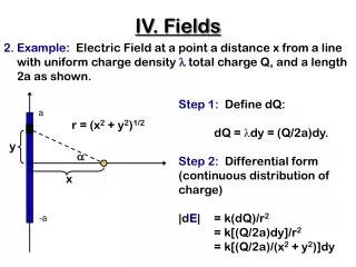
using using for The electric field on the axis of a finite line charge From Coulomb’s law The magnitude of the net electric field is the integral over each piece:
using using Beginning again with Coulomb’s law for the infinitesimal piece of charge: The magnitude of the electric field in the y-direction: Integrating: Finally, withx= y tan q
We can extend the result to an infinite line charge by lettingq = - p/2 and q = p/2 1 2 Using our previous results for the electric field due to a finite line charge Using Q = l L interchangeably
Example, Electric Field of a Charged Circular Rod Our element has a symmetrically located (mirror image) element ds in the bottom half of the rod. If we resolve the electric field vectors of ds and ds’ into x and y components as shown in we see that their y components cancel (because they have equal magnitudes and are in opposite directions).We also see that their x components have equal magnitudes and are in the same direction. Fig. 22-11 (a) A plastic rod of charge Q is a circular section of radius r and central angle 120°; point P is the center of curvature of the rod. (b) The field components from symmetric elements from the rod.
using Element along x integrating
Example Ring of Charge A ring of charge with the radius of 2 m, has an uniform distribution of charge of 1 nC. a) Find the electric field at x = 5m on an axis perpendicular and through the center of the ring b) What is x corresponding to the maximum E? c) What is the maximum E?
From the previous example of a ring of charge we know: Using dq = s dA = s 2p a da Doing the integration (and minus this for x<0)
Letting R/x >> 1 The electric field is discontinuous
NOTE: It is true in general that E is discontinuous at a surface of charge Look at a small enough disk and it can be treated as a uniform disk of charge. Consider a point P on the axis nd so close that the uniform disk appears infinite, then our previous result holds:
Example An infinitely long line of charge with λ = 0.6 µC/m lies along the z axis, and a point charge of q = 8 µC lies at y = 3m. Find the electric field at x = 4 m. E from line: q E from point charge: 5m 3m EL θ + 4m EP E Epx = Epcosθ = 2880 x 4/5 = 2304 N/C Epy = Epsinθ = -2880 x 3/5 = -1728 N/C Ey = -1728 N/C Ex = 2700 + 2304 = 5004 N/C E = 5294 N/C
Gauss’ Law: The first Maxwell Equation Chapter 23 Particularly useful in highly symmetric situations allowing derivation of the electric field More general than Coulomb’s Law We can move beyond static, point charge distributions We’ll derive Gauss’ Law for a static, point charge and then pose a heuristic argument for its validity in general
Electric Flux Φ • Flux (in general): Shows the flow of a quantity through a surface area. Electric Flux: proportional to the # of lines of field that penetrate the surface. # of lines that exit the surface enclosing the dipole = # of lines that enter the surface. Net flux = 0. # of lines that exit is the same as for a single charge +q.
With the area vector given by and is a unit vector perpendicular to the surface Electric Flux Definition electric field (constant) En θ A Only the perpendicular component En = E cosθ penetrates the surface and produces flux. The parallel component EII “glides” on the surface and causes no flux. the previous formula is exactly the dot product between:
Notice that for the flux is positive. While for the flux is negative So we can define the electric flux through a surface of area A The electric flux can be thought of as measuring the number of electric field lines penetrating a surface Field lines directed out of the surface make a positive contribution to the flux while field lines directed into the surface make a negative contribution to the flux
The flux projects out the component of the electric field perpendicular to the surface Equivalently, the flux projects out the component of the area perpendicular to the electric field:
Flux through a closed surface with the source of the field outside the surface = 0.
If we make the area element small enough, E will be constant across the element and the electric flux is: Imagine a tiny element of a surface with normal vector To find the flux across the entire surface we sum the individual pieces
For the purposes of Gauss’ Law, we’re interested in the flux through a closed surface
From Coulomb’s Law we know Imagine a sphere of radius R centered on Q Consider a point positive charge Q The net flux around the closed surface of the sphere is given by This is Gauss’s Law
Will often see Coulomb’s constant replaced with the permittivity of free space
Gauss’s Law Gauss’s law relates the electric flux ΦE through a closed surface to the net chargeqin that is inside that surface. • ΦEdoes not depend on • the location(s) of the charge(s) within the closed surface. • the shape of the closed (Gaussian) surface.
Carl Friedrich Gauss 1777-1855 Yes it’s the same guy that gave you the Gaussian distribution and … To give you some perspective he was born 50 years after Newton died (1642-1727). Predicted the time and place of the first asteroid CERES (Dec. 31, 1801). Had the unit of magnetic field named after him and of course had much to do with the development of mathematics Ceres t= 4.6 year , d=4.6 Au
Example: What is the electric flux ΦE due to a charge of 1.0 mC located at the center of a sphere of radius 1.0 m? • Questions: • What would be the electric flux if the radius of the sphere were • halved? • doubled?
Charge Q at the Center of a Sphere: Єo= permittivity of free space = 8.85 x 10⁻¹² C2/(N m2)
Gauss’s Law • Things to note: • We could have used any surface • Gauss’ Law is true in general
Gauss’ Law in E& M • Uses symmetry to determine E-field due to a charge distribution • Method: Considers a hypothetical surface enclosing some charge and calculates the E-field • The shape of that surface is “EVERYTHING”
KEY TO USING Gauss’s Law • The shape of the surrounding surface is one that MIMICS the symmetry of the charge distribution …..
This surface encloses q1, q2, but NOT q3. What is the net flux out of this surface? Answer:
Applied Gauss’ Law to Determine E-field in Cases where have • Spherical symmetry • Cylindrical symmetry • Planar symmetry
Gauss’ Law: Determining the E-field near the surface of a nonconducting (insulating) sheet To use Gauss’ Law choose symmetrical surfaces From the flux definition: We found the same E using Coulomb’s Law
Gauss’ Law: Determining the E-field near the surface of a nonconducting (insulating) sheet
Electric Field at surface of conductor is perpendicular to the surface and proportional to the charge density at the surface Shown that the excess charge resides on the outer surface of conductor surface. Unless the surface is spherical the charge density s (chg. per unit area) varies However the E-field just outside of a conducting surface is easy to determine using Gauss’ Law
In the figure bellow, an infinite plane of surface density σ = +4.5 nC/m2 lies in the x = 0 plane, and a second infinite plane of surface density σ = -4.5 nC/m2 lies at x = 2m, and is parallel to the first plane. a) Find the electric field at x = 1.8 m. 1) The plane at x = 0 produces the field: 2) The plane at x = 1.8 m produces the same field: 254 N/C 3) The total field Etot = 254 N/C + 254 N/C = 508 N/C b) Find the electric field at x = 5 m. 4) At x = 5m, the fields are in opposite directions: Etot = 254 N/C – 254 N/C = 0 N/C
Draw a spherical surface of radius Use Gauss’ Law to find E due to a spherical shell of charge Q This is just Coulomb’s Law
The symmetry is the same as before so we again have To find the field inside the shell draw another Gaussian surface, a sphere with However, this time, the charge enclosed is 0 so that,
Graphical Representation of E due to a spherical shell of charge Q
A uniformly charged solid sphere Find the E outside r >R
A uniformly charged solid sphere Find the E inside, r < R. or