Efficient Sketch-based Algorithms for String Collection Selection Queries
700 likes | 725 Views
Learn about sketch-based algorithms for efficient selection queries on string collections. Explore methods like transformation/synonym selection, sketch indexing, and weighted sets for approximate similarity computations.

Efficient Sketch-based Algorithms for String Collection Selection Queries
E N D
Presentation Transcript
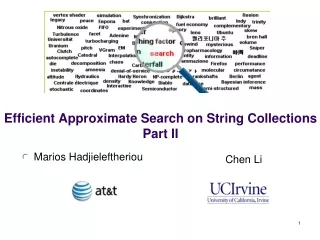
Efficient Approximate Search on String CollectionsPart II • Marios Hadjieleftheriou Chen Li
Overview • Sketch based algorithms • Compression • Selectivity estimation • Transformations/Synonyms
What is a Sketch • An approximate representation of the string • With size much smaller than the string • That can be used to upper bound similarity (or lower bound the distance) • String shas sketch sig(s) • If Simsig(sig(s), sig(t)) < θ, prune t • And Simsig is much more efficient to compute than the actual similarity of s and t
Using Sketches for Selection Queries • Naïve approach: • Scan all sketches and identify candidates • Verify candidates • Index sketches: • Inverted index • LSH (Gionis et al.) • The inverted sketch hash table (Chakrabarti et al.)
Known sketches • Prefix filter (CGK06) • Jaccard, Cosine, Edit distance • Mismatch filter (XWL08) • Edit distance • Minhash (BCFM98) • Jaccard • PartEnum (AGK06) • Hamming, Jaccard
Prefix Filter • Construction • Let string s be a set of q-grams: • s = {q4, q1, q2, q7} • Sort the set (e.g., lexicographically) • s = {q1, q2, q4, q7} • Prefix sketch sig(s) = {q1, q2} • Use sketch for filtering • If |s t| θ then sig(s) sig(t)
Example • Sets of size 8: s = {q1, q2, q4, q6, q8, q9, q10, q12} t = {q1, q2, q5, q6, q8, q10, q12, q14} • st = {q1, q2, q6, q8, q10, q12}, |st| = 6 • For any subset t’ t of size 3: s t’ • In worst case we choose q5, q14, and ?? • If |st|θ then t’ t s.t. |t’||s|-θ+1, t’ s 3 4 5 7 8 9 10 12 13 15 1 2 6 11 14 s … t
Example continued • Instead of taking a subset of t, we sort and take prefixes from both s and t: • pf(s) = {q1, q2, q4} • pf(t) = {q1, q2, q5} • If |s t| 6 then pf(s) pf(t) • Why is that true? • Best case we are left with at most 5 matching elements beyond the elements in the sketch
α w(s)-α pf(s) sf(s) Generalize to Weighted Sets • Example with weighted vectors • w(st) θ ( w(st) = Σqstw(q) ) • Sort by weights (not lexicographically anymore) • Keep prefix pf(s) s.t. w[pf(s)] w(s) - α w1 w2 … w14 1’ 2’ 4’ 6’ 8’ 10’ 12’ 14’ 0 w1 w2 0 w5 s t w5 w2 0 w3 0 Σqsf(s) w(q) = α
Continued • Best case: w[sf(s)sf(t)] = α • In other words, the suffixes match perfectly • w(st) = w[pf(s) pf(t)] + w[sf(s) sf(t)] • Consider the prefix and the suffix separately • w(st) θ w[pf(s) pf(t)] + w[sf(s) sf(t)]θ w[pf(s) pf(t)] θ - w[sf(s) sf(t)] • To avoid false negatives, minimize rhs w[pf(s) pf(t)] >θ - α
α w(s)-α pf(s) sf(s) Properties • w[pf(s) pf(t)] θ – α • Hence θ α • Hence α = θmin • Small θmin long prefix large sketch • For short strings, keep the whole string • Prefix sketches easy to index • Use Inverted Index
How do I Choose α? • I need |pf(s) pf(t)| w[pf(s) pf(t)] 0 θ = α
Extend to Jaccard • Jaccard(s, t) = w(s t) / w(s t) θ w(s t ) θ w(s t) • w(s t) = w(s) + w(t) – w(s t) … w[pf(s) pf(t)] β - w(sf(s) sf(t)] β = θ / (1 + θ) [w(s) + w(t)] • To avoid false negatives: w[pf(s) pf(t)] >β - α
Technicality w[pf(s) pf(t)] >β – α β = θ / (1 + θ) [w(s) + w(t)] • β depends on w(s), which is unknown at prefix construction time • Use length filtering • θ w(t) ≤ w(s) ≤ w(t) / θ
Extend to Edit Distance • Let string s be a set of q-grams: • s = {q11, q3, q67, q4} • Now the absolute position of q-grams matters: • Sort the set (e.g., lexicographically) but maintain positional information: • s = {(q3, 2), (q4, 4), (q11, 1), (q67, 3)} • Prefix sketch sig(s) = {(q3, 2), (q4, 4)}
Edit Distance Continued • ed(s, t) θ: • Length filter: abs(|s| - |t|) θ • Position filter: Common q-grams must have matching positions (within θ) • Count filter: s and t must have at least β = [max(|s|, |t|) – Q + 1] – Q θ Q-grams in common s = “Hello” has 5-2+1 2-grams • One edit affects at most q q-grams “Hello” 1 edit affects at most 2 2-grams
Edit Distance Candidates • Boils down to: • Check the string lengths • Check the positions of matching q-grams • Check intersection size: |s t| ≥ β • Very similar to Jaccard
α (|s|-q+1)-α pf(s) sf(s) Constructing the Prefix • |s t| max(|s|, |t|) – q + 1 – qθ … |pf(s) pf(t)| >β – α β = max(|s|, |t|) – q + 1 – qθ A total of (|s| - q + 1) q-grams
Choosing α |pf(s) pf(t)| >β – α β = max(|s|, |t|) – q + 1 – qθ • Set β = α • |pf(s)| ≥ (|s|-q+1) - α |pf(s)| = qθ+1 q-grams • If ed(s, t) ≤ θ thenpf(s) pf(t)
Pros/Cons • Provides a loose bound • Too many candidates • Makes sense if strings are long • Easy to construct, easy to compare
Mismatch Filter • When dealing with edit distance: • Position of mismatching q-grams within pf(s), pf(t) conveys a lot of information • Example: • Clustered edits: • s = “submit by Dec.” • t = “submit by Sep.” • Non-clustered edits: • s = “sabmit be Set.” • t = “submit by Sep.” 4 mismatching 2-grams 2 edits can fix all of them 6 mismatching 2-grams Need 3 edits to fix them
Mismatch Filter Continued • What is the minimum edit operations that cause the mismatching q-grams between s and t? • This number is a lower-bound on ed(s, t) • It is equal to the minimum edit operations it takes to destroy every mismatching q-gram • We can compute it using a greedy algorithm • We need to sort q-grams by position first (n logn)
Mismatch Condition • Fourth edit distance pruning condition: • Mismatched q-grams in prefixes must be destroyable with at most θ edits
Pros/Cons • Much tighter bound • Expensive (sorting), but prefixes relatively short • Needs long prefixes to make a difference
Minhash • So far we sort q-grams • What if we hash instead? • Minhash construction: • Given a string s = {q1, …, qm} • Use k functions h1, …, hk from independent family of hash functions,hi: q [0, 1] • Hash s, k times and keep the k q-grams q that hash to the smallest value each time • sig(s) = {qmh1, qmh2, …, qmhk}
How to use minhash • Example: • s = {q4, q1, q2, q7} • h1(s) = { 0.01, 0.87, 0.003, 0.562} • h2(s) = { 0.23, 0.15, 0.93, 0.62} • sig(s) = {0.003, 0.15} • Given two sketches sig(s), sig(t): • Jaccard(s, t) is the percentage of hash-values in sig(s) and sig(t) that match • Probabilistic: (ε, δ)-guarantees False negatives
Pros/Cons • Has false negatives • To drive errors down, sketch has to be pretty large • long strings • Will give meaningful estimations only if actual similarity between two strings is large • good only for large θ
PartEnum • Lower bounds Hamming distance: • Jaccard(s, t) θ H(s, t) 2|s| (1 – θ) / (1 + θ) • Partitioning strategy based on pigeonhole principle: • Express strings as vectors • Partition vectors into θ + 1 partitions • If H(s, t) θ then at least one partition has hamming distance zero. • To boost accuracy create all combinations of possible partitions
Example Partition sig1 sig2 Enumerate sig3 sig(s) = h(sig1) h(sig2) …
Pros/Cons • Gives guarantees • Fairly large sketch • Hard to tune three parameters • Actual data affects performance
A Global Approach • For disk resident lists: • Cost of disk I/O vs Decompression tradeoff • Integer compression • Golomb, Delta coding • Sorting based on non-integer weights?? • For main memory resident lists: • Lossless compression not useful • Design lossy schemes
Simple strategies • Discard lists: • Random, Longest, Cost-based • Discarding lists tag-of-war: • Reduce candidates: ones that appear only in the discarded lists disappear • Increase candidates: Looser threshold θ to account for discarded lists • Combine lists: • Find similar lists and keep only their union
Combining Lists • Discovering candidates: • Lists with high Jaccard containment/similarity • Avoid multi-way Jaccard computation: • Use minhash to estimate Jaccard • Use LSH to discover clusters • Combining: • Use cost-based algorithm based on query workload: • Size reduction • Query time reduction • When we meet both budgets we stop
General Observation • V-grams, sketches and compression use the distribution of q-grams to optimize • Zipf distribution • A small number of lists are very long • Those lists are fairly unimportant in terms of string similarity • A q-gram is meaningless if it is contained in almost all strings
The Problem • Estimate the number of strings with: • Edit distance smaller than θ • Cosine similarity higher than θ • Jaccard, Hamming, etc… • Issues: • Estimation accuracy • Size of estimator • Cost of estimation
Flavors • Edit distance: • Based on clustering (JL05) • Based on min-hash (MBK+07) • Based on wild-card q-grams (LNS07) • Cosine similarity: • Based on sampling (HYK+08)
Edit Distance • Problem: • Given query string s • Estimate number of strings t D • Such that ed(s, t) θ
Clustering - Sepia • Partition strings using clustering: • Enables pruning of whole clusters • Store per cluster histograms: • Number of strings within edit distance 0,1,…,θ from the cluster center • Compute global dataset statistics: • Use a training query set to compute frequency of data strings within edit distance 0,1,…,θ from each query • Given query: • Use cluster centers, histograms and dataset statistics to estimate selectivity
Minhash - VSol • We can use Minhash to: • Estimate Jaccard(s, t) = |st| / |st| • Estimate the size of a set |s| • Estimate the size of the union |st|
q1 q2 … q10 1 3 1 5 5 8 Inverted list … … … 14 25 43 Minhash VSol Estimator • Construct one inverted list per q-gram in D and compute the minhash sketch of each list:
Selectivity Estimation • Use edit distance count filter: • If ed(s, t) θ, then s and t share at least β = max(|s|, |t|) - q + 1 – qθ q-grams • Given query t = {q1, …, qm}: • We have m inverted lists • Any string contained in the intersection of at least β of these lists passes the count filter • Answer is the size of the union of all non-empty β-intersections (there are m choose β intersections)
q1 q2 … q14 t = 1 3 1 5 5 8 … … … 14 25 43 Example • θ = 2, q = 3, |t|=14 β = 6 • Look at all subsets of size 6 • Α = |{ι1, ..., ι6}(10 choose 6)(ti1 ti2 … ti6)| Inverted list
The m-β Similarity • We do not need to consider all subsets individually • There is a closed form estimation formula that uses minhash • Drawback: • Will overestimate results since many β-intersections result in duplicates
OptEQ – wild-card q-grams • Use extended q-grams: • Introduce wild-card symbol ‘?’ • E.g., “ab?” can be: • “aba”, “abb”, “abc”, … • Build an extended q-gram table: • Extract all 1-grams, 2-grams, …, q-grams • Generalize to extended 2-grams, …, q-grams • Maintain an extended q-grams/frequency hashtable
q-gram table q-gram Frequency ab 10 Dataset bc 15 string de 4 ef 1 sigmod gh 21 vldb hi 2 icde … … … ?b 13 a? 17 ?c 23 … … abc 5 def 2 … … Example
Assuming Replacements Only • Given query q=“abcd” • θ=2 • There are 6 base strings: • “??cd”, “?b?d”, “?bc?”, “a??d”, “a?c?”, “ab??” • Query answer: • S1={sD: s ”??cd”}, S2={sD: s ”?b?d”}, S3={…}, …, S6={…} • A = |S1 S2 S3 S4 S5 S6|= Σ1n6 (-1)n-1 |S1 … Sn|
Replacement Intersection Lattice A = Σ1n6 (-1)n-1 |S1 … Sn| • Need to evaluate size of all 2-intersections, 3-intersections, …, 6-intersections • Use frequencies from q-gram table to compute sum A • Exponential number of intersections • But ... there is well-defined structure