Download
1 / 44
440 likes | 558 Views
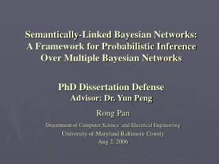
Semantically-Linked Bayesian Networks: A Framework for Probabilistic Inference Over Multiple Bayesian Networks PhD Dissertation Defense Advisor: Dr. Yun Peng. Rong Pan Department of Computer Science and Electrical Engineering University of Maryland Baltimore County Aug 2, 2006. Outline.

E N D
Semantically-Linked Bayesian Networks: A Framework for Probabilistic Inference Over Multiple Bayesian NetworksPhD Dissertation DefenseAdvisor: Dr. Yun Peng Rong Pan Department of Computer Science and Electrical Engineering University of Maryland Baltimore County Aug 2, 2006
Outline • Motivations • Background • Overview • How Knowledge is Shared • Inference on SLBN • Concept Mapping using SLBN • Future works
Motivations (1) • Separately developed BNs about • related domains • different aspects of the same domain …
Motivations (2) • Existing approach: • Multiply Sectioned Bayesian Networks (MSBN) Sectioning • Every subnet is sectioned from a global BN • Strictly consistent subnets • Exactly identical shared variables with same distribution • All parents of the shared variables must appear in one subnet
Motivations (3) • Existing approach: • Agent Encapsulated Bayesian Networks (AEBN) Output Variable Agent Input Variable Local Variable • Distribution BN Model for a specific application • Hierarchical global structure • Very restricted expressiveness • Exactly identical shared variables with different prior distributions
Motivations (4) • A distributed BN model was expected with features: • Uncertainty reasoning over separately developed BNs • Variables shared by different BNs can be similar but not identical • Principled, well justified • Support various applications
BackgroundBayesian Network • DAG • Variables • with Finite States • Edges: causal influences • Conditional Probability Table (CPT)
BackgroundEvidences in BN Soft Evidence: Q(Male_Mammal) = (0.5 0.5) Original BN Hard Evidence: Male_Mammal = True Virtual Evidence: L(Male_Mammal) = 0.8/0.2 Virtual Evidence = Soft Evidence: L(Male_Mammal) = 0.3/0.2
BackgroundJeffrey’s Rule (Soft Evidence) • Given external observations Q(Bi), the rest of the BN is updated by Jeffrey’s Rule: where P(A| Bi) is the conditional probability before evidence, Q(Bi) is the soft evidence. • Multiple Soft Evidences • Problem: update one variable’s distribution to its target value can make those of others’ off their targets • Solution: IPFP
BackgroundIterative Proportional Fitting Procedure (IPFP) • Q0 : initial distribution on the set of variables X, • {P(Si)}: a consistent set of n marginal probability distributions, where XSi. • The IPFP process where i is the iteration number, j = (i-1) mod n + 1 • The distribution after IPFP satisfies the given constraints {P(Si)} and has minimum cross-entropy to the initial distribution Q0
SLBN: Overview (1) • Semantically-Linked Bayesian Networks (SLBN) • A theoretical framework that supports probabilistic inference over separately developed BNs Global Knowledge Similar variables
SLBN: Overview (2) • Features • Inference over separate BNs that share semantically similar variables • Global knowledge: J-graph • Principled, well-justified • In SLBN • BNs are linked at the similar variables • Probabilistic influences are propagated via the shared variables • Inference process utilizes Soft Evidence (Jeffrey’s Rule), Virtual Evidence, IPFP, and traditional BN inference
How knowledge is shared:Semantic Similarity (1) What is similarity? Similar: Pronunciation: 'si-m&-l&r, 'sim-l&r Function:adjective 1: having characteristics in common 2: alike in substance or essentials 3: not differing in shape but only in size or position –– www.merrian-webster.com High-tech Company Employee V.S. High-income People Computer Keyboard V.S. Typewriter
How knowledge is shared:Semantic Similarity (2) • Semantic Similarity of concepts • Share of common instances • Quantified and utilized with direction • Quantified by the ratio of the shared instances to all the instances • Natural language’s definition for “similar” is vague • Hard to formalize • Hard to quantify • Hard to utilize in intelligence Conditional Probability P(High-tech Company Employee | High-income People)
How knowledge is shared:Variable Linkage (1) • In Bayesian Network (BN) / SLBN • Concepts are represented by variables • Semantic similarities are between propositions Man V.S.Woman We say “High-tech Company Employee” is similar to “High-income People” We mean “High-tech Company Employee = True” is similar to “High-income People = True”
How knowledge is shared:Variable Linkage (2) • Variable linkages • Represent semantic similarities in SLBN • Are between variables in different BNs A : Source Variable B : Destination Variable NA: Source BN NB: Destination BN : Quantification of the similarity is a m× n matrix:
How knowledge is shared:Variable Linkage (3) • Variable Linkage V.S. BN Edge
How knowledge is shared:Variable Linkage (4) • Expressiveness of Variable Linkage • Logical relationships defined in OWL syntax: Equivalent, Union, Intersection, and Subclass complement. • Relaxation of logical relationships by replacing set inclusion by overlapping: Overlap, Superclass, Subclass • Equivalence relations but same concepts are modeled as different variables
How knowledge is shared:Examples (1) Identical … Union …
How knowledge is shared:Examples (2) Overlap Superclass …
How knowledge is shared:Consistent Linked Variables • The priori beliefs on the linked variables on both sides must be consistent with the variable linkage: • P2(B) = ∑i PS(B|A=ai)P1(A=ai) • There exists a single distribution consistent with the prior belief on A, B, A, B, and the linkage’s similarity. • examined by IPFP P1(A) P1(A| A) P1(A) P2(B) P2(B| A) P2(B) A B A B PS(B| A)
Inference on SLBN The Process 3. Enter Soft/Virtual Evidences; 2. Propagate 1. Enter Evidence 4. Updated Result BN Belief Update With traditional Inference SLBN Rules for Probabilistic Influence Propagation BN Belief Update with Soft Evidence
Inference on SLBN The Theory Theoretical Basis Implementation (Existing) Implementation (SLBN) Bayes’ Rule Jeffrey’s Rule IPFP BN Inference Virtual Evidence Soft Evidence SLBN
Inference on SLBN Assumptions/Restrictions • All linked BNs are consistent with the linkages • One variable can only be involved in one linkage • Causal precedence in all linked BNs are consistent Linked BNs with consistent causal sequences Linked BNs with inconsistent causal sequences
Inference on SLBN Assumptions/Restrictions (Cont.) • For a variable linkage, the causes/effects of source is also the causes/effects of the destination • Linkages cannot cross each other … … … ... Crossed linkages
Inference on SLBN SLBN Rules for Probabilistic Influence Propagation (1) • Some hard evidence influence the source from bottom … • Propagated influences are represented by soft evidences • Beliefs of destination BN are update with SE Y1 X1 Y3 Y2 …
Inference on SLBN SLBN Rules for Probabilistic Influence Propagation (2) • Some hard evidence influence the source from top … • Additional soft evidences are created to cancel the influences from the linkage to parent(dest(L)) Y1 X1 Y3 Y2 …
Inference on SLBN SLBN Rules for Probabilistic Influence Propagation (3) • Some hard evidence influence the source from both top and bottom … • Additional soft evidences are created to propagate the combined influences from the linkage to parent(dest(L)) Y1 X1 Y3 Y2 …
Inference on SLBN Belief Update with Soft Evidence (1) • Represent soft evidences by virtual evidences • Belief update with soft evidence is IPFP • Belief update with one virtual evidence is one step of IPFP • Therefore, we can • Use virtual evidence to implement IPFP on BN • Use virtual evidence to implement soft evidence • SE VE • Iterate on the whole BN • Iterate on soft evidence variables
Inference on SLBN Belief Update with Soft Evidence (2) • Iterate on whole BN Q(A) = (0.6, 0.4) Q(B) = (0.5, 0.5) A B ve ve ve ve
Inference on SLBN Belief Update with Soft Evidence (1) • Iterate on SE variables P(A, B) = Q(A) = (0.6, 0.4) Q(B) = (0.5, 0.5) IPFP with Q(A), Q(B) A B Q(A, B) = ve
Inference on SLBN Belief Update with Soft Evidence (3) • Existing approaches : Big-Clique Iteration on whole BN: Small BNs, many soft evidences Iteration on se variables: Large BNs, a few soft evidences C: the big clique V: se variables |C|≥|V|
J-Graph (1)Overview • Joint-graph (J-graph) is a graphical probability model that represents • The joint distribution of SLBN • The interdependencies between variables across variable linkages • Usage • Check if all assumptions are satisfied • Justify Inference Process
J-Graph (2)Definition • J-Graph is constructed by merging all linked BNs and linkages into one graph • DAG • Variable nodes, Linkage Nodes • Edges: all edges in the linked BNs have a representation in J-graph • CPT: Q(A|A) = P(A|A), Q(A|B) = PS(A|B) for • Q: distribution in J-graph, P: original distribution
J-Graph (3)Example A’ A A1 A’2 B’ C’ B→B’; 1→2 C→C’; 1→2 B C Linkage Node D D’ D2 D’2 • Linkage nodes • represent all linked variables and the linkage • encode the similarity of the linkage in CPT • merge the CPTs by IPFP
Concept Mapping using SLBN (1)Motivations • Ontology mappings are seldom certain • Existing approaches • use hard threshold to filter mappings • throw similarities away after mappings are created • mappings are identical and 1-1 • But • often one concept is similar to more than one concept • Semantically similar concepts are hard to be represented logically
Concept Mapping using SLBN (2)The Framework WWW Onto1 Onto2 Learner Probabilistic Information BayesOWL BayesOWL BN1 BN2 Variable Linkages SLBN
Concept Mapping using SLBN (3)Objection • Discover new and complex concept mappings • Make full use of the learned similarity in SLBN’s inference • Create an expression for a concept in another ontology • Find how similar “Onto1:B Onto1:C” is to “Onto2:A” • Experiments have shown encouraging results
Concept Mapping using SLBN (3)Experiment • Artificial Intelligence sub-domain from ACM Topic Taxonomy DMOZ (Open Directory) hierarchies Learned Similarities: J(dmoz.sw, acm.rs) = 0.64 J(dmoz.sw, acm.sn) = 0.61 J(dmoz.sw, acm.krfm) = 0.49 After SLBN Inference: Q (acm.rs = True acm.sn = True | dmoz.sw = True) = 0.9646 J(dmoz.sw, acm.rs acm.sn) = 0.7250
Future Works • Modeling with SLBN • Discover semantic similar concepts by machine learning algorithms • Create effective and correct linkages from learned algorithms • Distributed Inference methods • Loosing the restrictions • Inference with linkages of both directions • Use functions to represent similarities
Thank You! • Questions?
Chain rule where(ai) is the parent set of ai. d-separation: BackgroundSemantics of BN d-separated variables do not influence each other. A B A C B Instantiated B A C C Not instantiated serials converging diverging