Lecture 8,9 – Linear Methods for Classification
Lecture 8,9 – Linear Methods for Classification. Rice ELEC 697 Farinaz Koushanfar Fall 2006. Summary. Bayes Classifiers Linear Classifiers Linear regression of an indicator matrix Linear discriminant analysis (LDA) Logistic regression Separating hyperplanes Reading (ch4, ELS).

Lecture 8,9 – Linear Methods for Classification
E N D
Presentation Transcript
Lecture 8,9 – Linear Methods for Classification Rice ELEC 697 Farinaz Koushanfar Fall 2006
Summary • Bayes Classifiers • Linear Classifiers • Linear regression of an indicator matrix • Linear discriminant analysis (LDA) • Logistic regression • Separating hyperplanes • Reading (ch4, ELS)
Bayes Classifier • The marginal distributions of G are specified as PMF pG(g), g=1,2,…,K • fX|G(x|G=g) shows the conditional distribution of X for G=g • The training set (xi,gi),i=1,..,N has independent samples from the joint distribution fX,G(x,g) • fX,G(x,g) = pG(g)fX|G(x|G=g) • The loss of predicting G* for G is L(G*,G) • Classification goal: minimize the expected loss • EX,GL(G(X),G)=EX(EG|XL(G(X),G))
Bayes Classifier (cont’d) • It suffices to minimize EG|XL(G(X),G) for each X. The optimal classifier is: • G(x) = argmin gEG|X=xL(g,G) • The Bayes rule is also known as the rule of maximum a posteriori probability • G(x) = argmax gPr(G=g|X=x) • Many classification algorithms estimate the Pr(G=g|X=x) and then apply the Bayes rule Bayes classification rule
More About Linear Classification • Since predictor G(x) take values in a discrete set G, we can divide the input space into a collection of regions labeled according to classification • For K classes (1,2,…,K), and the fitted linear model for k-th indicator response variable is • The decision boundary b/w k and l is: • An affine set or hyperplane: • Model discriminant function k(x) for each class, then classify x to the class with the largest value for k(x)
Linear Decision Boundary • We require that monotone transformation of k or Pr(G=k|X=x) be linear • Decision boundaries are the set of points with log-odds=0 • Prob. of class 1: , prob. of class 2: 1- • Apply a transformation:: log[/(1- )]=0+ Tx • Two popular methods that use log-odds • Linear discriminant analysis, linear logistic regression • Explicitly model the boundary b/w two classes as linear. For a two-class problem with p-dimensional input space, this is modeling decision boundary as a hyperplane • Two methods using separating hyperplanes • Perceptron - Rosenblatt, optimally separating hyperplanes - Vapnik
Generalizing Linear Decision Boundaries • Expand the variable set X1,…,Xp by including squares and cross products, adding up to p(p+1)/2 additional variables
Linear Regression of an Indicator Matrix • For K classes, K indicators Yk, k=1,…,K, with Yk=1, if G=k, else 0 • Indicator response matrix
Linear Regression of an Indicator Matrix (Cont’d) • For N training data, form NK indicator response matrix Y, a matrix of 0’s and 1’s • A new observation is classified as follows: • Compute the fitted output (K vector) - • Identify the largest component and classify accordingly: • But… how good is the fit? • Verify kG fk(x)=1 for any x • fk(x) can be negative or larger than 1 • We can allow linear regression into basis expansion of h(x) • As the size of training set increases, adaptively add more basis
Linear Regression - Drawback • For K3, especially for large K
Linear Regression - Drawback • For large K and small p, masking can naturally occur • E.g. Vowel recognition data in 2D subspace, K=11, p=10 dimensions
Linear Regression and Projection* • A linear regression function (here in 2D) • Projects each point x=[x1 x2]T to a line parallel to W1 • We can study how well the projected points {z1,z2,…,zn}, viewed as functions of w1, are separated across the classes * Slides Courtesy of Tommi S. Jaakkola, MIT CSAIL
Linear Regression and Projection • A linear regression function (here in 2D) • Projects each point x=[x1 x2]T to a line parallel to W1 • We can study how well the projected points {z1,z2,…,zn}, viewed as functions of w1, are separated across the classes
Projection and Classification • By varying w1 we get different levels of separation between the projected points
Optimizing the Projection • We would like to find the w1 that somehow maximizes the separation of the projected points across classes • We can quantify the separation (overlap) in terms of means and variations of the resulting 1-D class distribution
Fisher Linear Discriminant: Preliminaries • Class description in d • Class 0: n0 samples, mean 0, covariance 0 • Class 1: n1 samples, mean 1, covariance 1 • Projected class descriptions in • Class 0: n0 samples, mean 0Tw1, covariance w1T0 w1 • Class 1: n1 samples, mean 1Tw1, covariance w1T1 w1
Fisher Linear Discriminant • Estimation criterion: find w1 that maximizes • The solution (class separation) is decision theoretically optimal for two normal populations with equal covariances (1=0)
Linear Discriminant Analysis (LDA) • k class prior Pr(G=k) • Function fk(x)=density of X in class G=k • Bayes Theorem: • Leads to LDA, QDA, MDA (mixture DA), Kernel DA, Naïve Bayes • Suppose that we model density as a MVG: • LDA is when we assume the classes have a common covariance matrix: k= k. It’s sufficient to look at log-odds
LDA • Log-odds function implies decision boundary b/w k and l: Pr(G=k|X=x)=Pr(G=l|X=x) – linear in x; in p dimensions a hyperplane • Example: three classes and p=2
LDA (Cont’d) • In practice, we do not know the parameters of Gaussian distributions. Estimate w/ training set • Nk is the number of class k data • For two classes, this is like linear regression
QDA • If k’s are not equal, the quadratic terms in x remain; we get quadratic discriminant functions (QDA)
QDA (Cont’d) • The estimates are similar to LDA, but each class has a separate covariance matrices • For large p dramatic increase in parameters • In LDA, there are (K-1)(p+1) parameters • For QDA, there are (K-1){1+p(p+3)/2} • LDA and QDA both work really well • This is not because the data is Gaussian, rather, for simple decision boundaries, Gaussian estimates are stable • Bias-variance trade-off
Regularized Discriminent Analysis • A compromise b/w LDA and QDA. Shrink separate covariances of QDA towards a common covariance (similar to Ridge Reg.)
Computations for LDA • Suppose we compute the eigen decomposition for k, i.e. • Uk is pp orthonormal, Dkdiagonal matrix of positive eigenvalues dkl. Then, • The LDA classifier is implemented as: • X* D-1/2UTX, where =UDUT. The common covariance estimate of X* is identity • Classify to the closest class centroid in the transformed space, modulo the effect of the class prior probabilities k
Background: Simple Decision Theory* • Suppose we know the class-conditional densities p(X|y) for y=0,1 as well as the overall class frequencies P(y) • How do we decide which class a new example x’ belongs to so as to minimize the overall probability of error? * Courtesy of Tommi S. Jaakkola, MIT CSAIL
Background: Simple Decision Theory • Suppose we know the class-conditional densities p(X|y) for y=0,1 as well as the overall class frequencies P(y) • How do we decide which class a new example x’ belongs to so as to minimize the overall probability of error?
2-Class Logistic Regression • The optimal decisions are based on the posterior class probabilities P(y|x). For binary classification problems, we can write these decisions as • We generally don’t know P(y|x) but we can parameterize the possible decisions according to
2-Class Logistic Regression (Cont’d) • Our log-odds model • Gives rise to a specific form for the conditional probability over the labels (the logistic model): Where Is a logistic squashing function That turns linear predictions into probabilities
2-Class Logistic Regression: Decisions • Logistic regression models imply a linear decision boundary
K-Class Logistic Regression • The model is specified in terms of K-1 log-odds or logit transformations (reflecting the constraint that the probabilities sum to one) • The choice of denominator is arbitrary, typically last class …..
K-Class Logistic Regression (Cont’d) • The model is specified in terms of K-1 log-odds or logit transformations (reflecting the constraint that the probabilities sum to one) • A simple calculation shows that • To emphasize the dependence on the entire parameter set ={10, 1T,…,(K-1)0, T(K-1)}, we denote the probabilities as Pr(G=k|X=x) = pk(x; )
Fitting Logistic Regression Models • IRLS is equivalent to Newton-Raphson procedure
Fitting Logistic Regression Models • IRLS algorithm (equivalent to Newton-Raphson) • Initialize . • Form Linearized response: • Form weights wi=pi(1-pi) • Update by weighted LS of zi on xi with weights wi • Steps 2-4 repeated until convergence
Example – Logistic Regression • South African Heart Disease: • Coronary risk factor study (CORIS) baseline survey, carried out in three rural areas. • White males b/w 15 and 64 • Response: presence or absence of myocardial infarction • Maximum likelihood fit:
Example – Logistic Regression • South African Heart Disease:
Logistic Regression or LDA? • LDA: • This linearity is a consequence of the Gaussian assumption for the class densities, as well as the assumption of a common covariance matrix. • Logistic model • They use the same form for the logit function
Logistic Regression or LDA? • Discriminative vs informative learning: • logistic regression uses the conditional distribution of Y given x to estimate parameters, while LDA uses the full joint distribution (assuming normality). • If normality holds, LDA is up to 30% more efficient; o/w logistic regression can be more robust. But the methods are similar in practice.
Separating Hyperplanes • Perceptrons: compute a linear combination of the input features and return the sign • For x1,x2 in L, T(x1-x2)=0 • *= /|| || normal to surface L • For x0 in L, Tx0= - 0 • The signed distance of any point x to L is given by
Rosenblatt's Perceptron Learning Algorithm • Finds a separating hyperplane by minimizing the distance of misclassified points to the decision boundary • If a response yi=1 is misclassified, then xiT+0<0, and the opposite for misclassified point yi=-1 • The goal is to minimize
Rosenblatt's Perceptron Learning Algorithm (Cont’d) • Stochastic gradient descent • The misclassified observations are visited in some sequence and the parameters updated • is the learning rate, can be 1 w/o loss of generality • It can be shown that algorithm converges to a separating hyperplane in a finite number of steps
Optimal Separating Hyperplanes • Problem