Download
1 / 48
480 likes | 568 Views
Risk Premiums in Interest Rates. Week 8 – October 12, 2005. Types of Risk. Holding-period yield risk Capital gains risk Reinvestment risk Default risk Non-payment of principal Delayed or reduced payments Sometimes viewed as embedded option (put) Call risks

E N D
Risk Premiums in Interest Rates Week 8 – October 12, 2005
Types of Risk • Holding-period yield risk • Capital gains risk • Reinvestment risk • Default risk • Non-payment of principal • Delayed or reduced payments • Sometimes viewed as embedded option (put) • Call risks • Call risks can be viewed as embedded options (call) • Liquidity or marketability risk • Often measured as bid-ask spread for traded securities
Holding Period Yield Risk • Bond price is function of expected cash flows and RADR, but usually bond traders define contractual cash flows and yields to maturity • Relationship between YTM and p is a curve defined by equation from last week
Holding Period Risk (cont’d) • Zero coupon default risk free bonds held to maturity will earn yield to maturity • If maturity equals holding period, no risk • Future wealth from coupon bonds depends on income from reinvested cash at rates not known now • Bonds which must be sold at end of holding period (maturity does not equal holding period) have risk of capital gains or losses
Measuring Holding-Period Risk • Price sensitivity of bonds is measured in terms of a bond price elasticity • This elasticity is called durationdenoted d1, which is widely used by bond traders and analysts and is often available on quote sheets
Example of Duration • Assume a 10-year 8% coupon bond is priced at 12% yield to maturity and has value of 77.4 and duration of 6.8 • If yields changed immediately from 12% to 10%, that is a 2/112 or 1.8% change in gross yield • The bond price should change about 1.8% * 6.8 = 12.1%
Duration as Time Measure • Macauley noted that maturity was not relevant measure of timing of payments of bonds and defined his own measure, duration • The definition of duration is (p. 192):
Duration has two interpretations • Elasticity of bond prices with respect to changes in one plus the yield to maturity • Weighted average payment date of cash flows (coupon and interest) from bonds • Duration measure • Can be modified to be a yield elasticity by dividing by (1+yield to maturity) • Can be redefined using term structure of yields (Fisher-Weil duration noted d2)
Alternative Duration Calculation • Duration is widely used by bond traders and fixed income portfolio managers • Duration values are available from information services like Bloomberg • Calculated is three ways • Macauley’s formula (but combersome) • Calculate two prices and rates, divide changes • Closed-form solution, e.g. Dietrich formulation:
Duration is an Approximation Derivative is used in calculating duration Price (Par=1.0) Actual price change Change predicted by duration 0 Yield to Maturity
Duration as Risk Measure • Good • Balances reinvestment yield risk against capital gains risk • Widely used and clear mathematical expression assessing holding-period yield risk • Bad • Approximation and theoretical issues • Convexity adjustment only approximate improvement
Default or Credit Risk Example of 8% 3-year bond with risk-adjusted discount rate (RADR) of 12%:
Effect of Credit Risk Change • RADR constant at 12%: • Note price and yield change • Could be a change in one industry or firm • Default risk could be diversified in this case
Pricing Default-Risky Bond • Discount expected cash flows (related to default probabilities) to obtain value • Default probabilities may be related to bond ratings • Change in default probability will change expected cash flows and yield to maturity • Risk-adjusted discount rate (RADR) may or may not change with change in default risk
Risk Premiums in RADRs • Diversifiable or avoidable risks • Hedge portfolios can reduce or eliminate • Unsystematic risks are not priced (do not increase discount rate) • Priced versus non-priced risk • Systematic risks are unavoidable • Risk aversion (declining marginal utility of wealth) is underlying assumption
Default Risk Premiums • Vary over the business cycle • Can be changes in default risk probabilities or in the market price of risk • Current default risk premiums are very high relative to historical experience • Development of bond markets internationally is believed to promise substantial growth and risk analysis of private borrowers will be very important
Liquidity Risk • Unusual securities in often cannot be sold readily • Reflected in dealers’ spreads • If no market makers, can only be estimated • Thin markets require price concessions for quick transactions despite intrinsic values • Examples • Structured notes and Orange County • Drexel Burnam and junk bonds in 1980s • The Russian debt market collapse in 1998
Developments in Credit-risk • Usual interpretation of credit risk is default on a loan or bond • New views of credit risk are focused on the change in the credit-worthiness of debt instruments as well as default • Risk changes will be reflected in the value of a portfolio over time as write-downs or downgrades short of default reduce value of claims
Default • Private debt (corporate and household) may not pay cash flows as promised • Late payments • Nonpayment of interest or principal • Other default or credit events • Violation of covenants and other creditor interventions in operations • Change in risk of default (e.g. highly leveraged transactions)
Credit Events • Probability of default (PD) can change affecting the value of default-risky securities • Upgrades and downgrades reflecting changes in PD are credit events • Recent progress has been made in quantifying these probabilities
Bond and Debt Ratings • Rating agencies • Standard and Poor’s (AAA to D) • Moody’s (Aaa to C) • Fitch and Duff and Phelps • Migration of ratings, e.g. from BBB to BB (investment grade to below investment grade) represents credit risk • For example, change from BBB to BB has historical probability of 5.3% (S&P, 1996)
Risk of Fixed Incomes Probability Maximum value=F Future Value of Debt
Credit Losses • Three elements in credit losses • Estimated default probability (PD) • Loss given default (LGD) • Exposure at default (EAD) • Credit losses = PD*LGD*EAD • Investors in debt securities will be concerned about all these elements in managing their risks
Credit Risk Analysis • Credit risk has become a major focus of rating agencies, regulators, and investors • Very important to capital market development (e.g. asset securitizations, loan syndications) • Enron, Global Crossing, and GE exemplify different stages of concern with these issues • Consulting industry in credit analysis • RiskMetrics (formerly J.P. Morgan) • KMV (academic based research) • Others (KPMG, PricewaterhouseCoopers, etc.)
Example of Steps to estimate PD • Default occurs when value of assets less than value of liabilities (insolvency) • Example of analysis used by KMV uses simplified estimates of variables • Must calculate market value of assets (market value of debt and equity) and variability of market value • Identify book value of liabilities
Motorola: Debt and Equity Total Market Value
Distance to Default: Example • Motorola 2001-II (billions) Value of long-term debt = $ 7.3Book value of current liabilities = 12.9 Total value of liabilities = $20.2 Market value of assets = $56.6 Standard deviation of change in market value = 16.4% • Market value standard deviation of percent change = $9.3 billion
Reduced Probability of Default? • Estimated default point in example is midway between book value of current liabilities and long-term debt • Theory is that long-term debt does not require immediate payment, short-term liabilities may allow some flexibility • KMV uses historical data to fine-tune this estimate
Estimated Distance to Default Market value to default point = $40.0 $20.2 $56.6 $12.9 CL CL+LTD TMV Default point (estimated as midpoint) = $16.6
Distance to Default: 12-31-02 • Total Value of Assets (from “Capital Structure” and Financial Statements):E + LTD + CL = TA$33.9 + $ 8.1 + $9.7 = $ 51.7 • Book value of LTD and CL $8.4 and $9.7Midpoint estimate of default point = $13.9Std Dev = 16.4% * $51.7 = $8.48
Probability of Default • KMV has used historical data to relate distance from default to probability of default • That measure is proprietary (not available) • As example, Motorola is rated A3 by Standard and Poors, historically associated with a default rate of about .82% over next five years
Credit Risk in Portfolios • Individual assets have probability of default and risk and discussed last week • Loans in portfolios will have an interdependent risk structure due to correlations in defaults • Credit risk within portfolio context is a major advance in credit risk management • Search for a summary measure of portfolio risk led to the concept of value at risk
Value at Risk(VAR) • Value at risk (VAR) looks at risk of portfolio accounting for covariance of assets • Risk is defined in terms of likelihood of losses
Portfolio Credit Risk • Credit risk different than usual portfolio risk analysis • Returns are not symmetric • Concentrations of exposure complicate losses • Major issue is correlation of defaults and losses given default • We will discuss approach followed by CreditMetrics • Other approaches exist (including KMV)
Credit Risk as Rating Changes • Increased credit risk Default CCC B BB • Same credit risk (BBB) BBB A AA AAA • Less credit risk
Rating Migrations (BBB rating) Source: Standard & Poors
Probability of Default: Two Firms Value of Firm B Probability = 1/2% Probability = 1/10% Probability = 1/100% Default Point B Value of Firm A Default Point A
Simplified “Road Map” Compute exposure profile Of each asset Compute the volatility Of value caused by Up (down)grades and defaults Compute correlations Portfolio value-at-risk due to credit Source: Introduction to CreditMetrics (1997)
Required Resources • Default probabilities (or ratings) • Migration probabilities • Historical data requirements • Approaches to estimating correlations • Complete data on types of credits and estimations of losses given defaults • Exposures to classes of risks • Models and simulations of value changes given credit events
Credit Portfolio Risk One Asset Many Assets Frequency Frequency 0 0 Return Return
Incremental Risk • Introduction to CreditMetrics provides good examples (in Section 5) • Importance portfolio risk is the marginal risk • Marginal risk considers portfoliorisk implications 10% High risk and large size $ 10mm $ Credit Exposure
Next Week – October 19, 2005 • Take-home midterm examination due; 90-minute examination is open book and open note • Examination must be completed without discussion with anyone and a declaration to that effect and time spent turned in with examination • Prepare Chapter 9 • Arrange a meeting regarding project progress if you have not talked to me