MN20211: Corporate Finance 2009/10: Revision: Investment Appraisal, Portfolio, CAPM (AB).

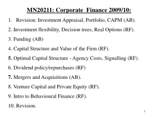
1. MN20211: Corporate Finance 2009/10: • Revision: Investment Appraisal, Portfolio, CAPM (AB). • 2. Investment flexibility, Decision trees, Real Options (RF). • 3. Funding (AB) • 4. Capital Structure and Value of the Firm (RF). • 5. Optimal Capital Structure - Agency Costs, Signalling (RF). • 6. Dividend policy/repurchases (RF) • 7. Mergers and Acquisitions (AB). • 8. Venture Capital and Private Equity (RF). • 9. Intro to Behavioural Finance (RF). • 10. Revision.

2. The Major Decisions of the Firm. • Investment Appraisal (Capital Budgeting) – Which New Projects to invest in? • Capital Structure (Financing Decision)- How to Finance the new projects – Debt or equity? • Payout Policy – Dividends, Share Repurchases, Re-investment. • => Objective: Maximisation of Shareholder Wealth.

3. 1. Investment Appraisal. • Objective: Take projects that increase shareholder wealth (Value-adding projects). • Investment Appraisal Techniques: NPV, IRR, Payback, ARR, Real Options…. • Which one is the Best rule for shareholder wealth maximisation?

4. Connections in Corporate Finance. Investment Appraisal: Net Present Value with discount rate (cost of capital) given. Positive NPV increases value of the firm. Cost of Capital (discount rate): How do companies derive the cost of capital? – CAPM/APT. Capital Structure and effect on Firm Value and WACC.

5. SECTION 1: Investment Appraisal. Debate over Correct Method - Accounting Rate of Return. - Payback. - NPV. - IRR. - POSITIVE NPV Increases Shareholder Wealth. 2. Correct Method - NPV! -Time Value of Money - Discounts all future cashflows

6. Net Present Value Perpetuities. IRR => Take Project if NPV > 0, or if IRR > r.

7. Example. Consider the following new project: -initial capital investment of £15m. -it will generate sales for 5 years. - Variable Costs equal 70% of sales value. - fixed cost of project £200k PA. - A feasibility study, cost £5000, has already been carried out. Discount Rate equals 12%. Should we take the project?

8. DO WE INVEST IN THIS NEW PROJECT? NPV > 0. COST OF CAPITAL (12%) < IRR (19.75%).

9. Note that if the NPV is positive, then the IRR exceeds the Cost of Capital. NPV £m 3.3m Discount Rate % 0 12 % 19.7%

10. CONFLICT BETWEEN APPRAISAL TECHNIQUES.

11. COMPARINGNPVANDIRR - 1 NPV 531 519 10% 22.8% 25.4% Discount Rate PROJ D PROJ C Select Project with higher NPV: Project C.

12. COMPARINGNPVANDIRR -2 NPV Discount Rate Impossible to find IRR!!! NPV exists!

13. COMPARINGNPVANDIRR –3 Size Effect Discount Rate: 10% Project A : Date 0 Investment -£1000. Date 1 Cashflow £1500. NPV = £364. IRR = 50% Project B:- Date 0 Investment -£10 Date 1 Cashflow £18. NPV = £6.36 IRR = 80%. Which Project do we take?

14. Mutually Exclusive Versus Independent Projects. • Mutually Exclusive project: firm can only take one (take project with highest positive NPV). • Independent project: firm can take as many as it likes (take all positive NPV projects). • Consider slide 10: Which project(s) would you take, and what would be the value-added, if projects are a) mutually exclusive, and b) independent?

15. Which Cash-flows to use? • Economic costs and revenues: ie take the cash when it occurs. (see depreciation treatment). • Relevant Cashflows. • Incremental cashflows. • => NPV is a measure of value-creation for shareholders from taking new project.

16. Treatment of depreciation.

17. Lecture 3: Investment Flexibility, Decision Trees, and Real Options • Decision Trees and Sensitivity Analysis. • Example: From RWJ. • New Project: Test and Development Phase: Investment $100m. • 0.75 chance of success. • If successful, Company can invest in full scale production, Investment $1500m. • Production will occur over next 5 years with the following cashflows.

18. Production Stage: Base Case Date 1 NPV = -1500 + = 1517

19. Decision Tree. Date 1: -1500 Date 0: -$100 NPV = 1517 Invest P=0.75 Success Do not Invest NPV = 0 Test Do not Invest Failure P=0.25 Do Not Test Invest NPV = -3611 Solve backwards: If the tests are successful, SEC should invest, since 1517 > 0. If tests are unsuccessful, SEC should not invest, since 0 > -3611.

20. Now move back to Stage 1. Invest $100m now to get 75% chance of $1517m one year later? Expected Payoff = 0.75 *1517 +0.25 *0 = 1138. NPV of testing at date 0 = -100 + = $890 Therefore, the firm should test the project. Sensitivity Analysis (What-if analysis or Bop analysis) Examines sensitivity of NPV to changes in underlying assumptions (on revenue, costs and cashflows).

21. Sensitivity Analysis. - NPV Calculation for all 3 possibilities of a single variable + expected forecast for all other variables. Limitation in just changing one variable at a time. Scenario Analysis- Change several variables together. Mosher Case study. Break - even analysis examines variability in forecasts. It determines the number of sales required to break even.

22. EVA (Economic Value Added). • EVA developed, and trade-marked, by Stern and Stewart. • EVA closely related to NPV • But NPV = investment decision rule, forward-looking expected value-creation over life of a project. • EVA is an ongoing Annual Performance Evaluation Technique. • Rewards managers on annual value-creation.

23. Section 6: Options as Financial Building Blocks. A call option gives the holder the right (but not the obligation) to buy shares at some time in the future at an exercise price agreed now. A put option gives the holder the right (but not the obligation) to sell shares at some time in the future at an exercise price agreed now. European Option – Exercised only at maturity date. American Option – Can be exercised at any time up to maturity. For simplicity, we focus on European Options.

24. Factors Affecting Price of European Option (=c). • -Underlying Stock Price S. • -Exercise Price X. • Variance of of the returns of the underlying asset , • Time to maturity, T. The riskier the underlying returns, the greater the probability that the stock price will exceed the exercise price. The longer to maturity, the greater the probability that the stock price will exceed the exercise price.

25. Combining options, graphic presentation. Buying a Call Option. Selling a put option. Selling a Call Option. Buying a Put Option.

26. Long in Stock Buy a Bond Sell a Bond Short in Stock S + P = B + C. S + P – C = B. Other Combinations: Spread, Straddle, Straps and strips. See Exercise.

27. Equity as a Call Option. Black and Scholes pointed out that equity is a call option on the value of the levered firm. If Value of firm exceeds face value of debt (exercise price of call option), equityholders pay the exercise price, and gain the increase in value. If value of firm is less than face value of debt, option is not exercised. Risky debt = risk-free debt – put option (B – P).

28. Building Blocks. S + P = B + C : for Option. V + P = B + S: for levered firm. => V = (B – P) + S. S = Max [ 0, V – D ]. Equity = call option. B – P = Min [ V, D ]. Risky debt = risk free debt – put option. Therefore, V = ( B – P ) + S. S B-P V V D D

29. Important Implications for Firm. Equity is a call option: Value of Equity in creases with risk. Value of Put option increases with risk: Therefore value of debt decreases with risk. After all, Equity holders have limited liability, and S = Max [ 0, V – D ]. B – P = Min [ V, D ]. With (B – P) + S = V. Therefore, if S increases, ( B – P) decreases. Equity holders will want to choose riskier projects.

30. Pricing Call Options – Binomial Approach. Cu = 3 uS=24.00 q q c S=20 1- q 1- q dS=13.40 Cd=0 • S = £20. q=0.5. u=1.2. d=.67. X = £21. • 1 + rf = 1.1. • Risk free hedge Portfolio: Buy One Share of Stock and write m call options. • uS - mCu = dS – mCd => 24 – 3m = 13.40. • M = 3.53. By holding one share of stock, and selling 3.53 call options, your payoffs are the same in both states of nature (13.40): Risk free.

31. Since hedge portfolio is riskless: 1.1 ( 20 – 3.53C) = 13.40. Therefore, C = 2.21. This is the current price per call option. The total present value of investment = £12 .19, and the rate of return on investment is 13.40 / 12.19 = 1.1.

32. Application of Options- Convertible Debt. • Convertible Debt gives the holder the right (but not the obligation) to convert bonds into equity at a future date. • Convertible debt is a combination of straight debt plus a call option. • We saw that straight debt = risky debt – a put option. • CD = D + C = B – P + C . • Implication: Value of Convertible debt increases with risk of firm’s cashflows, and time to maturity. • -See CD exercise. • more detailed analysis of convertible debt in 4th year advanced finance course.

33. EVA with constant invested capital. • Project with Initial required Capital Investment • Capital Lasts forever (no depreciation). • Project generates cashflow in each future period n.

34. EVA example. • Consider an investment opportunity requiring initial investment of 250 (no depreciation). • Project is expected to produce perpetuity of 35 (ie annually forever). • Discount rate

35. EVA Example • EVA of investment opportunity in every year is • Present Value of these EVAs is

36. Real Options. • Real Options recognise flexibility in investment appraisal decision. • Standard NPV: static; “now or never”. • Real Option Approach: “Now or Later”. • -Option to delay, option to expand, option to abandon. • Analogy with financial options (later in course).

37. Types of Real Option • Option to Delay (Timing Option). • Option to Expand (eg R and D). • Option to Abandon.

38. Valuation of Real Options • Binomial Pricing Model • Black-Scholes formula

39. Value of a Real Option • A Project’s Value-added = Standard NPV plus the Real Option Value. • For given cashflows, standard NPV decreases with risk (why?). • But Real Option Value increases with risk. • R and D very risky: => Real Option element may be high.

40. Simplified Examples • Option to Expand (page 241 of RWJ) If Successful Expand Build First Ice Hotel Do not Expand If unsuccessful

41. Option to Expand (Continued) • NPV of single ice hotel • NPV = - 12,000,000 + 2,000,000/0.20 =-2m • Reject? • Optimistic forecast: NPV = - 12M + 3M/0.2 • = 3M. • Pessimistic: NPV = -12M + 1M/0.2 = - 7m • Still reject?

42. Option to expand (continued) • Given success, the E will expand to 10 hotels • => • NPV = 50% x 10 x 3m + 50% x (-7m) = 11.5 m. • Therefore, invest.

43. Option to abandon. • NPV(opt) = - 12m + 6m/0.2 = 18m. • NPV (pess) = -12m – 2m/0.2 = -22m. • => NPV = - 2m. Reject? • But abandon if failure => • NPV = 50% x 18m + 50% x -12m/1.20 • = 2.17m • Accept.

44. Option to delay and Competition (Smit and Ankum). • -benefit: wait to observe market demand. • -cost: Lost cash flows. • -cost: lost monopoly advantage, increasing competition. • Net Operating Cashflow = opportunity cost plus economic rent; Economic Rent: Innovation, barriers to entry, product differentiation, patents. Long-run: ER = 0. Firm needs too identify extent of competitive advantage.

45. Option to delay and Competition (Smit and Ankum) – Cont’d. Cash inflow during deferment period = In monopoly model: constant economic rent. In competition, economic rent declines to zero. -trade-off between option value of waiting, and loss from competition.

46. The Investment Appraisal Debate. Richard Pike: Sample size: 100 Large UK based Firms.

47. Combination of Techniques: Pike 1992: ( ) = NPV

48. Some Reasons for usage of wrong techniques. • -Managers prefer % figures => IRR, ARR • Managers don’t understand NPV/ Complicated Calculations. • Payback simple to calculate. • Short-term compensation schemes => Payback (Levy 200 –203, Pike 1985 pg 49). • Behavioural Factors (see later section on Behavioural Finance!!) • Increase in Usage of correct DCF techniques: • Computers. • Management Education.

49. SECTION 2: Risk and Return/Portfolio Decision/ Cost Of Capital. The cost of capital = investors’ required return on their investment in a company. It provides the appropriate discount rate in NPV. Investors are risk averse. Future share prices (and returns) are risky (volatile). The higher the risk, the higher the required return. p r A B t t

50. An investor’s actual return is the percentage change in price: Risk = Variability or Volatility of Returns, Var (R). We assume that Returns follow a Normal Distribution. Var(R). E(R)