Structured Prediction and Active Learning for Information Retrieval

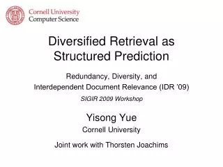
1. Structured Prediction and Active Learning for Information Retrieval Presented at Microsoft Research Asia August 21st, 2008 Yisong Yue Cornell University Joint work with: Thorsten Joachims (advisor), Filip Radlinski, Thomas Finley, Robert Kleinberg, Josef Broder

2. Outline • Structured Prediction • Complex Retrieval Goals • Structural SVMs (Supervised Learning) • Active Learning • Learning From Real Users • Multi-armed Bandit Problems

3. Supervised Learning x y 7.3 x x y y 1 -1 Microsoft announced today that they acquired Apple for the amount equal to the gross national product of Switzerland. Microsoft officials stated that they first wanted to buy Switzerland, but eventually were turned off by the mountains and the snowy winters… GATACAACCTATCCCCGTATATATATTCTATGGGTATAGTATTAAATCAATACAACCTATCCCCGTATATATATTCTATGGGTATAGTATTAAATCAATACAACCTATCCCCGTATATATATTCTATGGGTATAGTATTAAATCAGATACAACCTATCCCCGTATATATATTCTATGGGTATAGTATTAAATCACATTTA • Find function from input space X to output space Y such that the prediction error is low.

4. Examples of Complex Output Spaces Natural Language Parsing Given a sequence of words x, predict the parse tree y. Dependencies from structural constraints, since y has to be a tree. x The dog chased the cat y S NP VP NP Det N V Det N

5. Examples of Complex Output Spaces x The rain wet the cat y Det V Det N N • Part-of-Speech Tagging • Given a sequence of words x, predict sequence of tags y. • Dependencies from tag-tag transitions in Markov model. •  Similarly for other sequence labeling problems, e.g., RNA Intron/Exon Tagging.

6. Examples of Complex Output Spaces • Multi-class Labeling • Sequence Alignment • Grammar Trees & POS Tagging • Markov Random Fields • Clustering • Information Retrieval (Rankings) • Average Precision & NDCG • Listwise Approaches • Diversity • More Complex Goals

7. Information Retrieval • Input: x (feature representation of a document/query pair) • Conventional Approach • Real valued retrieval functions f(x) • Sort by f(xi) to obtain ranking • Training Method • Human-labeled data (documents labeled by relevance) • Learn f(x) using relatively simple criterion • Computationally convenient • Works pretty well (but we can do better)

8. Conventional SVMs Input: x (high dimensional point) Target: y (either +1 or -1) Prediction: sign(wTx) Training: subject to: The sum of slacks upper bounds the accuracy loss

9. Pairwise Preferences SVM Such that: Large Margin Ordinal Regression [Herbrich et al., 1999] Can be reduced to time [Joachims, 2005] Pairs can be reweighted to more closely model IR goals [Cao et al., 2006]

10. Mean Average Precision Consider rank position of each relevance doc K1, K2, … KR Compute Precision@K for each K1, K2, … KR Average precision = average of P@K Ex: has AvgPrec of MAP is Average Precision across multiple queries/rankings

11. Optimization Challenges • Rank-based measures are multivariate • Cannot decompose (additively) into document pairs • Need to exploit other structure • Defined over rankings • Rankings do not vary smoothly • Discontinuous w.r.t model parameters • Need some kind of relaxation/approximation

12. [Y & Burges; 2007]

13. Optimization Approach • Approximations / Smoothing • Directly define gradient • LambdaRank [Burges et al., 2006] • Gaussian smoothing • SoftRank GP [Guiver & Snelson, 2008] • Upper bound relaxations • Exponential Loss w/ Boosting • AdaRank [Xu et al., 2007] • Hinge Loss w/ Structural SVMs • [Chapelle et al., 2007] • SVM-map [Yue et al., 2007]

14. Structured Prediction Let x be a structured input (candidate documents) Let y be a structured output (ranking) Use a joint feature map to encode the compatibility of predicting y for given x. Captures all the structure of the prediction problem Consider linear models: after learning w, we can make predictions via

15. Linear Discriminant for Ranking • Let x = (x1,…xn) denote candidate documents (features) • Let yjk = {+1, -1} encode pairwise rank orders • Feature map is linear combination of documents. • Prediction made by sorting on document scores wTxi

16. Linear Discriminant for Ranking • Using pairwise preferences is common in IR • So far, just reformulated using structured prediction notation. • But we won’t decompose into independent pairs • Treat the entire ranking as a structured object • Allows for optimizing average precision

17. Structural SVM Let x denote a structured input (candidate documents) Let y denote a structured output (ranking) Standard objective function: Constraints are defined for each incorrect labeling y’ over the set of documents x. [Y, Finley, Radlinski, Joachims; SIGIR 2007]

18. Structural SVM for MAP Minimize subject to where ( yjk= {-1, +1} ) and Sum of slacks is smooth upper bound on MAP loss. [Y, Finley, Radlinski, Joachims; SIGIR 2007]

19. Too Many Constraints! For Average Precision, the true labeling is a ranking where the relevant documents are all ranked in the front, e.g., An incorrect labeling would be any other ranking, e.g., This ranking has Average Precision of about 0.8 with (y’) ¼ 0.2 Intractable number of rankings, thus an intractable number of constraints!

20. Structural SVM Training Original SVM Problem Intractable number of constraints Most are dominated by a small set of “important” constraints Structural SVM Approach Repeatedly finds the next most violated constraint… …until set of constraints is a good approximation. [Tsochantaridis et al., 2005]

21. Structural SVM Training Original SVM Problem Intractable number of constraints Most are dominated by a small set of “important” constraints Structural SVM Approach Repeatedly finds the next most violated constraint… …until set of constraints is a good approximation. [Tsochantaridis et al., 2005]

22. Structural SVM Training Original SVM Problem Intractable number of constraints Most are dominated by a small set of “important” constraints Structural SVM Approach Repeatedly finds the next most violated constraint… …until set of constraints is a good approximation. [Tsochantaridis et al., 2005]

23. Structural SVM Training Original SVM Problem Intractable number of constraints Most are dominated by a small set of “important” constraints Structural SVM Approach Repeatedly finds the next most violated constraint… …until set of constraints is a good approximation. [Tsochantaridis et al., 2005]

24. Finding Most Violated Constraint A constraint is violated when Finding most violated constraint reduces to Highly related to inference/prediction:

25. Finding Most Violated Constraint Observations MAP is invariant on the order of documents within a relevance class Swapping two relevant or non-relevant documents does not change MAP. Joint SVM score is optimized by sorting by document score, wTxj Reduces to finding an interleaving between two sorted lists of documents

26. Finding Most Violated Constraint Start with perfect ranking Consider swapping adjacent relevant/non-relevant documents ►

27. Finding Most Violated Constraint Start with perfect ranking Consider swapping adjacent relevant/non-relevant documents Find the best feasible ranking of the non-relevant document ►

28. Finding Most Violated Constraint Start with perfect ranking Consider swapping adjacent relevant/non-relevant documents Find the best feasible ranking of the non-relevant document Repeat for next non-relevant document ►

29. Finding Most Violated Constraint Start with perfect ranking Consider swapping adjacent relevant/non-relevant documents Find the best feasible ranking of the non-relevant document Repeat for next non-relevant document Never want to swap past previous non-relevant document ►

30. Finding Most Violated Constraint Start with perfect ranking Consider swapping adjacent relevant/non-relevant documents Find the best feasible ranking of the non-relevant document Repeat for next non-relevant document Never want to swap past previous non-relevant document Repeat until all non-relevant documents have been considered ►

32. Structural SVM for MAP • Treats rankings as structured objects • Optimizes hinge-loss relaxation of MAP • Provably minimizes the empirical risk • Performance improvement over conventional SVMs • Relies on subroutine to find most violated constraint • Computationally compatible with linear discriminant

33. Need for Diversity (in IR) Ambiguous Queries Users with different information needs issuing the same textual query “Jaguar” At least one relevant result for each information need Learning Queries User interested in “a specific detail or entire breadth of knowledge available” [Swaminathan et al., 2008] Results with high information diversity

34. Query: “Jaguar” Top of First Page Bottom of First Page Result #18 Results From 11/27/2007

35. Learning to Rank • Current methods • Real valued retrieval functions f(q,d) • Sort by f(q,di) to obtain ranking • Benefits: • Know how to perform learning • Can optimize for rank-based performance measures • Outperforms traditional IR models • Drawbacks: • Cannot account for diversity • During prediction, considers each document independently

36. Example • Choose K documents with maximal information coverage. • For K = 3, optimal set is {D1, D2, D10}

37. Diversity via Set Cover • Documents cover information • Assume information is partitioned into discrete units. • Documents overlap in the information covered. • Selecting K documents with maximal coverage is a set cover problem • NP-complete in general • Greedy has (1-1/e) approximation [Khuller et al., 1997]

38. Diversity via Subtopics Current datasets use manually determined subtopic labels E.g., “Use of robots in the world today” Nanorobots Space mission robots Underwater robots Manual partitioning of the total information Relatively reliable Use as training data

39. Weighted Word Coverage • Use words to represent units of information • More distinct words = more information • Weight word importance • Does not depend on human labeling • Goal: select K documents which collectively cover as many distinct (weighted) words as possible • Greedy selection yields (1-1/e) bound. • Need to find good weighting function (learning problem).

40. Example Document Word Counts Marginal Benefit

41. Example Document Word Counts Marginal Benefit

42. Related Work Comparison • Essential Pages[Swaminathan et al., 2008] • Uses fixed function of word benefit • Depends on word frequency in candidate set • Our goals • Automatically learn a word benefit function • Learn to predict set covers • Use training data • Minimize subtopic loss • No prior ML approach • (to our knowledge)

43. Linear Discriminant • x = (x1,x2,…,xn) - candidate documents • y – subset of x • V(y) – union of words from documents in y. • Discriminant Function: • (v,x) – frequency features (e.g., ¸10%, ¸20%, etc). • Benefit of covering word v is thenwT(v,x) [Y, Joachims; ICML 2008]

44. Linear Discriminant • Does NOT reward redundancy • Benefit of each word only counted once • Greedy has (1-1/e)-approximation bound • Linear (joint feature space) • Allows for SVM optimization [Y, Joachims; ICML 2008]

45. More Sophisticated Discriminant Documents “cover” words to different degrees A document with 5 copies of “Microsoft” might cover it better than another document with only 2 copies. Use multiple word sets, V1(y), V2(y), … , VL(y) Each Vi(y) contains only words satisfying certain importance criteria. [Y, Joachims; ICML 2008]

46. More Sophisticated Discriminant • Separate i for each importance level i. • Joint feature map  is vector composition of all i • Greedy has (1-1/e)-approximation bound. • Still uses linear feature space. [Y, Joachims; ICML 2008]

47. Weighted Subtopic Loss • Example: • x1 covers t1 • x2 covers t1,t2,t3 • x3 covers t1,t3 • Motivation • Higher penalty for not covering popular subtopics • Mitigates effects of label noise in tail subtopics

48. Structural SVM • Input: x (candidate set of documents) • Target: y (subset of x of size K) • Same objective function: • Constraints for each incorrect labeling y’. • Scoreof best y at least as large as incorrect y’ plus loss • Finding most violated constraint also set cover problem

49. TREC Experiments TREC 6-8 Interactive Track Queries Documents labeled into subtopics. 17 queries used, considered only relevant docs decouples relevance problem from diversity problem 45 docs/query, 20 subtopics/query, 300 words/doc

50. TREC Experiments 12/4/1 train/valid/test split Approx 500 documents in training set Permuted until all 17 queries were tested once Set K=5 (some queries have very few documents) SVM-div – uses term frequency thresholds to define importance levels SVM-div2 – in addition uses TFIDF thresholds