Balanced Search Trees: AVL and B-Trees
220 likes | 232 Views
Explore AVL trees and B-Trees, two types of balanced search trees. Learn the concept of height-balancing and how it affects insertion. Discover the benefits and limitations of using AVL trees and the heuristic approach of Splay trees.

Balanced Search Trees: AVL and B-Trees
E N D
Presentation Transcript
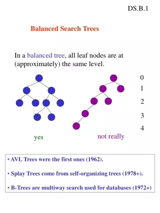
DS.B.1 Balanced Search Trees In a balanced tree, all leaf nodes are at (approximately) the same level. 0 1 2 3 4 not really yes • AVL Trees were the first ones (1962). • Splay Trees come from self-organizing trees (1978+). • B-Trees are multiway search used for databases (1972+)
DS.B.2 AVL Trees (Adelson-Velskii and Landis, 1962) AVL trees are binary search trees that are maintained as height-balanced. This means: • They are excellent for searching (log N). • There is extra work on insertion and deletion.
DS.B.3 Height-Balancing The balance-factor of a node of a binary search tree is: height(left subtree) - height(right subtree) A height-balanced tree has balance factor of -1, 0, or 1 at every node. That is, the height of the left and right subtrees of each node differ by at most 1. Examples:
DS.B.4 How does this affect insertion? Inserting a new node can cause a balanced tree to become unbalanced. But only those nodes on the path from the insertion point to the root can have their balances altered. We rebalance the tree by rebalancing the deepest such node. BF = 1 BF = 1 BF = 0 BF = 0 BF = 0 BF = 0 BF = 0 BF = 0 BF = 0 Tree before insertion.
DS.B.5 A new node is inserted. Which is the deepest node with |BF| > 1? Tree after insertion. BF = BF = BF = BF = BF = BF = BF = BF = BF = BF = 0
DS.B.6 Let the node that needs rebalancing be . There are 4 cases: Outside Cases (require single rotation) : - Insertion into left subtree of left child of . - Insertion into right subtree of right child of . Inside Cases (require double rotation) : - Insertion into right subtree of left child of . - Insertion into left subtree of right child of . The rebalancing is performed through four separate rotation algorithms.
DS.B.7 Should we always use AVL trees instead of ordinary binary search trees? Arguments for AVL trees: 1. Search is O(log N), since AVL trees are always balanced. 2. The height balancing adds no more than a constant factor to the speed of insertion. Arguments against always using AVL trees: 1. It’s nasty to program. 2. It IS SLOWER on most inserts (that constant of complexity thing). 3. Most large searches are done in database systems on DISK and use other structures. 4. Internal trees need not be always balanced.
DS.B.8 SPLAY TREES Splay trees are internal tree structures that 1. Are not perfectly balanced all the time 2. Let the actual retrievals force rebalancing that benefits future retrievals Using the heuristic: If X is accessed once, it is likely to be accessed again. • After node X is accessed, perform splaying • operations to bring it up to the root of the tree. • -Do this in a way that leaves the tree more • balanced as a whole.
DS.B.9 DETAILS • Let X be a nonroot node with 2 ancestors. • Let P be its parent node. • Let G be its grandparent node. G G G G P P P P X X X X Will X always have a P and a G?
DS.B.10 LINKED IMPLEMENTATION 1. Nodes must contain a parent pointer. element left right parent 2. There are actually six rotation routines. • Single Rotations (X has a P but no G) • Double Rotations (X has both a P and a G) • zig_left • zig_right • zig_zig_left • zig_zig_right • zig_zag_left • zig_zag_right
DS.B.11 COMPLEXITY OF SPLAYING The analysis is rather advanced and is in Chapter 11. We won’t cover it. Result of Analysis: Any m operations on a splay tree of size n take O(m log n) time. The amortized running time for one operation is O(log n). This guarantees that even if the depths of some nodes get very large, you can’t get a big sequence of O(n) searches, because each one causes a rebalance.
DS.B.12 B-Trees B-Trees are multi-way search trees commonly used in database systems or other applications where keeping the tree shallow is important. A B-Tree of order M has the following properties: 1. The root is either a leaf or has between 2 and M children. 2. All nonleaf nodes (except the root) have between M/2 and M children. 3. All nonroot leaf nodes have betweenM/2 and M keys. (*) 4. All leaves are at the same depth. (This is nice.) All data records are stored at (or more likely pointed to by) the leaves.
DS.B.13 B-Tree Nonleaf Node P[1] K[1] . . . K[i-1] P[i-1] K[i] . . . K[q-1] P[q] x y z K[q-1] z x < K[1] K[i-1]Y<K[i] • The Ks are keys • The Ps are pointers to subtrees.
DS.B.14 Leaf Node Structure K[1] R[1] . . . K[q-1] R[q-1] Next • The Ks are keys (assume unique). • The Rs are pointers to records with those keys. • The Next link points to the next leaf in key order. 75 89 95 103 115 95 Jones Mark 19 4 data record
DS.B.15 B-trees of order 4 are called 2-3-4 trees, because 1. Each nonleaf, nonroot node has 2, 3, or 4 children (1, 2, or 3 keys). 2. Each nonroot leaf node has 2, 3, or 4 keys. Try one.
DS.B.16 B-trees of order 3 are called 2-3 trees, because 1. Each nonleaf, nonroot node has 2 or 3 children (1or 2 keys). 2. Each nonroot leaf node has 2 or 3 keys. 7 5 9 15 1 2 3 5 6 7 8 9 12
DS.B.17 Searching a B-Tree T for a Key Value K Find(ElementType K, Btree B) { B = T; while (B is not a leaf) { find the Pi in node B that points to the proper subtree that K will be in; B = Pi; } /* Now we’re at a leaf */ if key K is the jth key in leaf B, use the jth record pointer to find the associated record; else /* K is not in leaf B */ report failure; } How would you search for a key in a node?
DS.B.18 Inserting a New Key in a B-Tree of Order M Insert(ElementType K, Btree B) { find the leaf node LB of B in which K belongs; if notfull(LB) insert K into LB; else { split LB into two nodes LB and LB2 with j = (M+1)/2 keys in LB and the rest in LB2; if ( IsNull(Parent(LB)) ) CreateNewRoot(LB, K[j+1], LB2); else InsertInternal(Parent(LB), K[j+1], LB2); } } LB LB2 K[1] R[1] . . . K[j] R[j] K[j+1] R[j+1] . . . K[M] R[M]
DS.B.19 Inserting a (Key,Ptr) Pair into an Internal Node If the node is not full, insert them in the proper place and return. If the node is already full (M pointers, M-1 keys), find the place for the new pair and split the adjusted (Key,Ptr) sequence into two internal nodes with j = (M+1)/2 pointers and j-1 keys in the first, the next key inserted in the node’s parent, and the rest in the second. K[j] P[1] K[1] . . . K[j-1] P[j] P[j+1] K[j+1] . . . K[M] P[M+1]
DS.B.20 DELETION When a record is deleted, remove it from its leaf node. If it also occurs in an internal node, remove it from there, too. Deletion may cause “underflow” if a node ends up with too few entries. • Strategies for underflow: • Try to redistribute entries from siblings • Lazy delete: just mark it gone.
DS.B.21 COMPLEXITY • Find: O(log N) (depth of tree) • Insert/Delete: O(M log N) M/2 M M
DS.B.22 How Do We Select the Order M? - In internal memory, small orders, like 3 or 4 are fine. - On disk, we have to worry about the number of disk accesses to search the index and get to the proper leaf. Rule: Choose the largest M so that an internal node can fit into one physical block of the disk. This leads to typical M’s between 32 and 256 And keeps the trees as shallow as possible.