Download
1 / 85
850 likes | 871 Views
Explore feedback applications for self-optimizing control and stabilization of new operating regimes by Sigurd Skogestad from NTNU. Learn about control structure design, anti-slug control, and more.

E N D
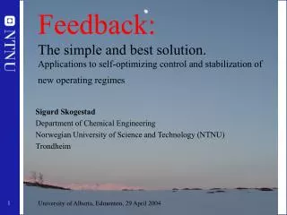
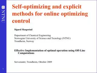
FeedbackApplications to self-optimizing control and stabilization of new operating regimes Sigurd Skogestad Department of Chemical Engineering Norwegian University of Science and Technlogy (NTNU) Trondheim South China University of Technology, Guangzhou, 05 January 2004
Outline • About myself • Example 1: Why feedback (and not feedforward) ? • What should we control? Secondary variables (Example 2) • What should we control? Primary controlled variables • A procedure for control structure design (plantwide control) • Example stabilizing control: Anti-slug control • Conclusion
Sigurd Skogestad • Born in 1955 • 1978: Siv.ing. Degree (MS) in Chemical Engineering from NTNU (NTH) • 1980-83: Process modeling group at the Norsk Hydro Research Center in Porsgrunn • 1983-87: Ph.D. student in Chemical Engineering at Caltech, Pasadena, USA. Thesis on “Robust distillation control”. Supervisor: Manfred Morari • 1987 - : Professor in Chemical Engineering at NTNU • Since 1994: Head of process systems engineering center in Trondheim (PROST) • Since 1999: Head of Department of Chemical Engineering • 1996: Book “Multivariable feedback control” (Wiley) • 2000,2003: Book “Prosessteknikk” (Norwegian) • Group of about 10 Ph.D. students in the process control area
Arctic circle North Sea Trondheim!! SWEDEN NORWAY Oslo DENMARK GERMANY UK
Research: Develop simple yet rigorous methods to solve problems of engineering significance. • Use of feedback as a tool to • reduce uncertainty (including robust control), • change the system dynamics (including stabilization; anti-slug control), • generally make the system more well-behaved (including self-optimizing control). • limitations on performance in linear systems (“controllability”), • control structure design and plantwide control, • interactions between process design and control, • distillation column design, control and dynamics. • Natural gas processes
Outline • About myself • Example 1: Why feedback (and not feedforward) ? • What should we control? Secondary variables (Example 2) • What should we control? Primary controlled variables • A procedure for control structure design (plantwide control) • Example stabilizing control: Anti-slug control • Conclusion
k=10 time 25 Example 1 1 d Gd G u y Plant (uncontrolled system)
d Gd G u y
Model-based control =Feedforward (FF) control d Gd G u y ”Perfect” feedforward control: u = - G-1 Gd d Our case: G=Gd → Use u = -d
d Gd G u y FF control: Nominal case (perfect model)
d Gd G u y FF control: change in gain in G
d Gd G u y FF control: change in time constant
d Gd G u y FF control: change in delay (in G or Gd)
d Gd ys e C G u y Measurement-based correction =Feedback (FB) control
d Gd ys e C G u y Output y Input u Feedback generates inverse! Resulting output Feedback PI-control: Nominal case
d Gd ys e C G u y Feedback PI control: change in gain in G
d Gd ys e C G u y FB control: change in time constant in G
d Gd ys e C G u y FB control: change in time delay in G
d Gd ys e C G u y FB control: all cases
d Gd G u y FF control: all cases
Comment • Time delay error in disturbance model (Gd): No effect (!) with feedback (except time shift) • Feedforward: Similar effect as time delay error in G
Why feedback?(and not feedforward control) • Counteract unmeasured disturbances • Reduce effect of changes / uncertainty (robustness) • Change system dynamics (including stabilization) • No explicit model required • MAIN PROBLEM • Potential instability (may occur suddenly)
Outline • About myself • Example 1: Why feedback (and not feedforward) ? • What should we control? Secondary variables (Example 2) • What should we control? Primary controlled variables • A procedure for control structure design (plantwide control) • Example stabilizing control: Anti-slug control • Conclusion
d u ys e G2 G1 C y Example 2: Plant with delay PI-control ys=1 d=6
Fundamental limitation feedback: Delay θ • Effective delay PI-control = ”original delay” + ”inverse response” + ”half of second time constant” + ”all smaller time constants”
Improve control? • Feedback: Some improvement possible with more complex controller • For example, add derivative action (PID-controller) • May reduce θeff from 5 s to 2 s • Problem: Sensitive to measurement noise • Does not remove the fundamental limitation • Feedforward: Good for time delay systems, but need model + measurement of disturbance. Sensitive to uncertainty. • Feedback cascade: Add extra measurement and introduce local control • May remove the fundamental limitation from high-order dynamics
ys y2 y2s u G2 G1 C1 C2 y Without cascade With cascade Cascade control w/ extra secondary measurement (2 PI’s) d
Cascade control • Inner fast (secondary) loop that control secondary variable: • P or PI-control • Local disturbance rejection • Much smaller effective delay (0.2 s) • Outer slower primary loop: • Reduced effective delay (2 s) • No loss in degrees of freedom • Setpoint in inner loop new degree of freedom • Time scale separation • Inner loop can be modelled as gain=1 + effective delay • Very effective for control of large-scale systems
Outline • About myself • Example 1: Why feedback (and not feedforward) ? • What should we control? Secondary variables (Example 2) • What should we control? Primary controlled variables • A procedure for control structure design (plantwide control) • Example stabilizing control: Anti-slug control • Conclusion
Process operation: Hierarchical structure RTO MPC Includes stabilizing control. As just shown: Can itself be hiearchical (cascaded) PID
Engineering systems • Most (all?) large-scale engineering systems are controlled using hierarchies of quite simple single-loop controllers • Commercial aircraft • Large-scale chemical plant (refinery) • 1000’s of loops • Simple components: on-off + P-control + PI-control + nonlinear fixes + some feedforward Same in biological systems
Alan Foss (“Critique of chemical process control theory”, AIChE Journal,1973): The central issue to be resolved ... is the determination of control system structure. Which variables should be measured, which inputs should be manipulated and which links should be made between the two sets?
y1 = c ? (economics) y2 = ? (cascade control) What should we control?
Optimal operation (economics) • Define scalar cost function J(u0,d) • u0: degrees of freedom • d: disturbances • Optimal operation for given d: minu0 J(u0,d) subject to: f(u0,d) = 0 g(u0,d) < 0
Active constraints • Optimal solution is usually at constraints, that is, most of the degrees of freedom are used to satisfy “active constraints”, g(u0,d) = 0 • CONTROL ACTIVE CONSTRAINTS! • Implementation of active constraints is usually simple. • WHAT MORE SHOULD WE CONTROL? • We here concentrate on the remaining unconstrained degrees of freedom u.
Optimal operation Cost J Jopt uopt Independent variable u (remaining unconstrained)
Implementation: How do we deal with uncertainty? • 1. Disturbances d • 2. Implementation error n us = uopt(d0) – nominal optimization n u = us + n d Cost J Jopt(d)
Problem no. 1: Disturbance d d ≠d0 Cost J d0 Jopt Loss with constant value for u uopt(d0) Independent variable u
Problem no. 2: Implementation error n Cost J d0 Loss due to implementation error for u Jopt us=uopt(d0) u = us + n Independent variable u
”Obvious” solution: Optimizing control Probem: Too complicated
Alternative: Feedback implementation Issue: What should we control?
Self-optimizing Control • Define loss: • Self-optimizing Control • Self-optimizing control is when acceptable loss can be achieved using constant set points (cs)for the controlled variables c (without re-optimizing when disturbances occur).
Constant setpoint policy: Effect of disturbances (“problem 1”)
Effect of implementation error (“problem 2”) Good Good BAD
Self-optimizing Control – Marathon • Optimal operation of Marathon runner, J=T • Any self-optimizing variable c (to control at constant setpoint)?
Self-optimizing Control – Marathon • Optimal operation of Marathon runner, J=T • Any self-optimizing variable c (to control at constant setpoint)? • c1 = distance to leader of race • c2 = speed • c3 = heart rate • c4 = level of lactate in muscles