DIRECTIONAL HYPOTHESIS
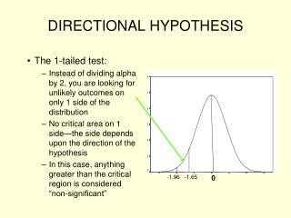
DIRECTIONAL HYPOTHESIS. The 1-tailed test: Instead of dividing alpha by 2, you are looking for unlikely outcomes on only 1 side of the distribution No critical area on 1 side—the side depends upon the direction of the hypothesis

DIRECTIONAL HYPOTHESIS
E N D
Presentation Transcript
DIRECTIONAL HYPOTHESIS • The 1-tailed test: • Instead of dividing alpha by 2, you are looking for unlikely outcomes on only 1 side of the distribution • No critical area on 1 side—the side depends upon the direction of the hypothesis • In this case, anything greater than the critical region is considered “non-significant” -1.96 -1.65 0
Non-Directional & Directional Hypotheses • Nondirectional • Ho: there is no effect: (X = µ) • H1: there IS an effect: (X ≠ µ) • APPLY 2-TAILED TEST • 2.5% chance of error in each tail • Directional • H1: sample mean is larger than population mean (X > µ) • Ho x ≤ µ • APPLY 1-TAILED TEST • 5% chance of error in one tail -1.96 1.96 1.65
Why we typically use 2-tailed tests • Often times, theory or logic does allow us to prediction direction – why not use 1-tailed tests? • Those with low self-control should be more likely to engage in crime. • Rehabilitation programs should reduce likelihood of future arrest. • What happens if we find the reverse? • Theory is incorrect, or program has the unintended consequence of making matters worse.
STUDENT’S t DISTRIBUTION • We can’t use Z distribution with smaller samples (N<100) because of large standard errors • Instead, we use the t distribution: • Approximately normal beginning when sample size > 30 • Probabilities under the t distribution are different than from the Z distribution for small samples • They become more like Z as sample size (N) increases
THE 1-SAMPLE CASE • 2 Applications • Single sample means (large N’s) (Z statistic) • May substitute sample s for population standard deviation, but then subtract 1 from n • s/√N-1 on bottom of z formula • Smaller N distribution (t statistic), population SD unknown
STUDENT’S t DISTRIBUTION • Find the t (critical) values in App. B of Healey • “degrees of freedom” • # of values in a distribution that are free to vary • Here, df = N-1 • When finding t(critical) always use lower df associated with your N Practice: ALPHA TEST N t(Critical) .05 2-tailed 57 .0 1 1-tailed 25 .10 2-tailed 32 .05 1-tailed 15
Example: Single sample means, smaller N and/or unknown pop. S.D. • A random sample of 26 sociology grads scored an average of 458 on the GRE sociology test, with a standard deviation of 20. Is this significantly higher than the national average (µ = 440)? • The same students studied an average of 19 hours a week (s=6.5). Is this significantly different from the overall average (µ = 15.5)? • USE ALPHA = .05 for both
1-Sample Hypothesis Testing (Review of what has been covered so far) • If the null hypothesis is correct, the estimated sample statistic (i.e., sample mean) is going to be close to the population mean 2. When we “set the criteria for a decision”, we are deciding how far the sample statistic has to fall from the population mean for us to decide to reject H0 • Deciding on probability of getting a given sample statistic if H0 is true • 3 common probabilities (alpha levels) used are .10, .05 & .01 • These correspond to Z score critical values of 1.65, 1.96 & 258
1-Sample Hypothesis Testing (Review of what has been covered so far) 3. If test statistic we calculate is beyond the critical value (in the critical region) then we reject H0 • Probability of getting test stat (if null is true) is small enough for us to reject the null • In other words: “There is a statistically significant difference between population & sample means.” 4. If test statistic we calculate does not fall in critical region, we fail to reject the H0 • “There is NOT a statistically significant difference…”
2-Sample Hypothesis Testing (intro) • Apply when… • You have a hypothesis that the means (or proportions) of a variable differ between 2 populations • Components • 2 representative samples – Don’t get confused here (usually both come from same “sample”) • One interval/ratio dependent variable • Examples • Do male and female differ in their aggression (# aggressive acts in past week)? • Is there a difference between MN & WI in the proportion who eat cheese every day? • Null Hypothesis (Ho) • The 2 pops. are not different in terms of the dependent variable
2-SAMPLE HYPOTHESIS TESTING • Assumptions: • Random (probability) sampling • Groups are independent • Homogeneity of variance • the amount of variability in the D.V. is about equal in each of the 2 groups • The sampling distribution of the difference between means is normal in shape
2-SAMPLE HYPOTHESIS TESTING • We rarely know population S.D.s • Therefore, for 2-sample t-testing, we must use 2 sample S.D.s, corrected for bias: • “Pooled Estimate” • Focus on the t statistic: t (obtained) = (X – X) σx-x • we’re finding the difference between the two means… …and standardizing this difference with the pooled estimate
2-SAMPLE HYPOTHESIS TESTING • 2-Sample Sampling Distribution • – difference between sample means (closer sample means will have differences closer to 0) • t-test for the difference between 2 sample means: • Addresses the question of whether the observed difference between the sample means reflects a real difference in the population means or is due to sampling error -2.042 0 2.042 ASSUMING THE NULL!
Applying the 2-Sample t Formula • Example: • Research Hypothesis (H1): • Soc. majors at UMD drink more beers per month than non-soc. majors • Random sample of 205 students: • Soc majors: N = 100, mean=16, s=1.0 • Non soc. majors: N = 105, mean=15, s=0.9 • Alpha = .01 • FORMULA: t(obtained) = X1 – X2 pooled estimate
Answers • Null hypothesis: • “There is no difference in mean number of fights between inmates with tattoos and inmates without tattoos.” • Use a 1 or 2-tailed test? • One-tailed test because the theory predicts that inmates with tattoos will get into MORE fights.
Answers • Calculations • Obtained value • Reject the null? • Yes because the t(obtained) (19.09) is greater than the t(critical, one-tail, df=398) (1.658) • This t value indicates there are 19.09 standard error units that separate the two mean values • VERY unlikely we got this big a difference due to sampling error • Research hypothesis restated as non-directional: • “There is a difference in the mean number of fights reported by inmates with tattoos and inmates without tattoos.” • Would you come to a different conclusion if you used a 2-tailed test? • No, because 19.09 is still well beyond the 2-tailed critical value (1.980).
2-Sample Hypothesis Testing in SPSS • Independent Samples t Test Output: • Testing the Ho that there is no difference in number of adult arrests between a sample of individuals who were abused/neglected as children and a matched control group.
Interpreting SPSS Output • Difference in mean # of adult arrests between those who were abused as children & control group
Interpreting SPSS Output • t statistic, with degrees of freedom
Interpreting SPSS Output • “Sig. (2 tailed)” • gives the actual probability of making a Type I (alpha) error • a.k.a. the “p value” – p = probability
“Sig.” & Probability • Number under “Sig.” column is the exact probability of obtaining that t-value (finding that mean difference) if the null is true • When probability > alpha, we do NOT reject H0 • When probability < alpha, we DO reject H0 • As the test statistics (here, “t”) increase, they indicate larger differences between our obtained finding and what is expected under null • Therefore, as the test statistic increases, the probability associated with it decreases
Example 2: Education & Ageat which First Child is Born H0: There is no relationship between whether an individual has a college degree and his or her age when their first child is born.
Education & Age at which First Child is Born • What is the mean difference in age? • What is the probability that this t statistic is due to sampling error? • Do we reject H0 at the alpha = .05 level? • Do we reject H0 at the alpha = .01 level?