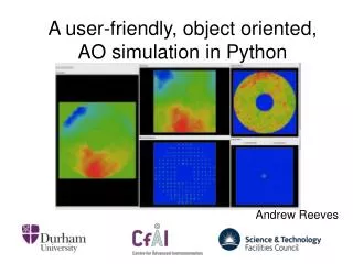
A user-friendly, object oriented, AO simulation in Python
A user-friendly, object oriented, AO simulation in Python. Andrew Reeves. Summary . Another AO Simulation….? Python Programming Language Simulation code Overview Examples of current investigations. Why another Simulation?. Written entirely in Python Object- Oriented Simulation “Toolkit”

A user-friendly, object oriented, AO simulation in Python
E N D
Presentation Transcript
A user-friendly, object oriented, AO simulation in Python Andrew Reeves
Summary • Another AO Simulation….? • Python Programming Language • Simulation code Overview • Examples of current investigations
Why another Simulation? • Written entirely in Python • Object-Oriented Simulation “Toolkit” • Easy to use • Rapid development and testing of new, complicated AO concepts • Learning tool to explore AO systems
Python • Interpreted, high-level, general purpose programming language. • Portable, works “out of the box” on Windows, Mac OS, Linux etc…. • Interpreter can be used interactively, with impressive interactive tools (matplotlib, ipython) • Object-oriented, but can be used as a functional language, or just for scripting • Enormous community support with packages available for almost anything with usage growing very quickly
Python Syntax Docstrings: Distinct from comments, these are used to document code as the code is written. Can be parsed by various tools to create documentation, or when “ help(function)” is called. Indentation: Code blocks are delimited by the indentation level, no {}s are required. Makes code very easy to read. • Python can be used to write Object-Oriented or functional code, or can be used simply to write scripts.
Python data-structures • Flexible data structures • “lists”, “dictionarys” and “tuples” • Can contain combinations of any type of data or object • Can be dynamically expanded/shrunk as required • list1 = ["helloWorld", 1, 10.67, aoSimObject, (10,10)] • NumPy Arrays • Multi-dimensional arrays of fixed size and type • Fast data access, with many fancy indexing techniques • array1 = numpy.array([1,2,3], [4,5,6]), slice = array1[1:2, :] • No explicit pointer syntax, though NumPy Arrays will pass pointers automatically and NumPy methods are available which make this more user controllable.
Python performance • Pure python isn’t very fast • But…….. • Many libraries exist which wrap fast C algorithms in python – especially for scientific purposes e.g. numPy, sciPy, matplotlib, pyfftw • Multi-processing is very easy • Tools such as Cython exist to accelerate pure python by converting to C and compiling. • C-Python API makes writing extensions in C easy.
Time solving 100 iterations of the Laplace Equation for a 500x500 grid. Code is still high-level, easy to understand Python! http://wiki.scipy.org/PerformancePython#head-a3f4dd816378d3ba4cbdd3d23dc98529e8ad7087
The Python AO Simulation • An AO simulation which uses many of pythons features to make it simple to understand and easy to use and expand. • AO components, such as WFSs, DMs, and reconstructors are modelled as self-contained objects, which act in an way which corresponds to the real world items. • Objects can be run in the existing simulation framework, or used independently. • A base class for most component types is available which deals with boiler-plate code. A new type of sub-system can be created quickly by inheriting the base and adding the new, interestingmethods. • Using external libraries, acceptable performance can be achieved.
Simulation Class Diagram Class name: Example Class Attributes: Example Class Methods:
Class A contains instances of Class B B A Class B inherits from Class A A B
Simulation Features • Multiple Wave-Front Sensors • Only Shack-Hartmann, but easy to create new types. • WFS objects stored in a python, so can be easily accessed and examined.
Simulation Features • Realistic Laser Guide Stars • Physical propagation of up-link path includes tip-tilt variations LGS uplink PSF Convolved WFS spots
Simulation Features • Realistic Laser Guide Stars • Elongation modelled by propagating multiple LGS layers at different heights 8m Primary, 6” subap FOV 32x32 subaps 90km Sodium Layer, 10km thickness 5 elongation layers, Uplink turbulence
Simulation Features • Using IPython console, can inspect and plot simulation data and change simulation parameters in real time
Simulation GUI, showing plotting of simulation data. Console can be used to inspect data and change parameters in real-time
Simulation Features • Multiprocessing for multiple WFSs • Each WFS assigned to a core. • Simple with python • Physical or geometric light propagation for WFSs and LGS. • Variety of reconstructors implemented, including Woofer-Tweeter, Learn and Apply, Artificial Neural Network • Simple configuration from Config file
Artificial Neural Networks • A potential tomographic reconstructor. • There is evidence to suggest that ANNs are robust against changing turbulence profiles. • ANN must be ``trained’’ on a generic data set, then can be used for any turbulence profile.
Artificial Neural Networks • Easy to adapt the simulation to use an ANN. • Sub-class the “Reconstructor” class, and override the “reconstruct” method • Parent “Reconstructor” takes care of all interfaces and boiler-plate code • Now simulation can use an ANN instead of traditional matrix based reconstructor
LGS Up-link Prediction • Possible to predict LGS up-link path using tomography? • If each WFS views the path through turbulence of other Lasers perhaps. • Only possible if up-link path is not reciprocal to path down….
Correlation of tip-tilt modes in up and down-link paths through Kolmogorov turbulence Correlation of tip-tilt is small for a small aperture concentric with the telescope aperture. DLLT/D: Ratio of LGS launch aperture size to telescope diameter (Wilson & Jenkins, 1996)
Correlation of tip-tilt modes in up and down-link paths through Kolmogorov turbulence Correlation of tip-tilt is small for a small aperture concentric with the telescope aperture. DLLT/D: Ratio of LGS launch aperture size to telescope diameter (Wilson & Jenkins, 1996)
LGS Up-link Prediction • If up-link and down-link tip-tilt uncorrelated, then slope measured on WFS is a combination of both effects Measured slope Component of slope due to down-link turbulence Component of slope due to up-link turbulence
LGS Up-link Prediction • If 2 LGS, α and β, the WFS β observes the up-link path of LGS α. • Can prove that there is a linear relationship between down-link only slopes sαt, and sβt and the slopes measured on a WFS sαand sβ. • With sαt, and sβtcan now reconstruct on-phase correction as usual. • Manuscript on the above in preparation α β H h … 0 n D
LGS Up-link Prediction • If 2 LGS, α and β, the WFS β observes the up-link path of LGS α. • Can prove that there is a linear relationship between down-link only slopes sαt, and sβt and the slopes measured on a WFS sαand sβ. • With sαt, and sβtcan now reconstruct on-phase correction as usual. • Manuscript on the above in preparation α β H h … 0 n D
LGS Up-link Prediction • Since relationship between up-link slopes and down-link turbulence slopes is linear, can use Learn & Apply algorithm (Vidal, Gendron & Rousset, 2010) • Relies on covariance matrices between off and on axis matrices. • Can simulate this with realistic LGS up-link turbulence using python AO sim. • LGS covariance on on-axis and 4 off-axis LGS for an 8x8 sub-aperture system • Note vertical and horizontal dark lines of negative correlation. NGS LGS1 LGS2 LGS3 LGS4 NGS LGS1 LGS2 LGS3 LGS4
Simulation Parameters • 512 phase points across aperture • 16x16 sub-aperture system • 17x17 actuator DM • 4 off-axis LGS WFSs on 10” square • LGS at height of 90km • uses on-axis NGS for “learn” step • 5 Layer Profile (shown right)
Results • Algorithm improves performance over no tip-tilt correction. • Not suited to high resolution imaging applications. • Ground layer not corrected well, NGS could still be required for Ground layer correction • Algorithm shows promise to improve GLAO performance for low resolution spectroscopy applications
Summary • Python is a great language for scientific applications, including AO simulations. • We have created a python AO simulation which can be run stand-alone, or used as a toolkit to quickly develop new AO ideas. • Simulation already contains many useful features such as multiple WFSs, realistic LGS and different reconstructors. • Code is under heavy development to increase features and performance. • Simulation already being used to develop new, novel, ideas for AO.

