Download
1 / 48
510 likes | 981 Views
Probabilistic Reasoning Systems - Introduction to Bayesian Network -. CS570 AI Team #7: T. M. Kim, J. B. Hur, H. Y. Park Speaker: Kim, Tae Min. Outline. Introduction to graphical model Review: Uncertainty and Probability Representing Knowledge in an Uncertain Domain

E N D
Probabilistic Reasoning Systems- Introduction to Bayesian Network - CS570 AI Team #7: T. M. Kim, J. B. Hur, H. Y. Park Speaker: Kim, Tae Min
Outline • Introduction to graphical model • Review: Uncertainty and Probability • Representing Knowledge in an Uncertain Domain • Semantics of bayesian Networks • Inference in bayesian Networks • Summary • Practice Questions • Useful links on the WWW
What is a graphical model? • A graphical model is a way of representing probabilistic relationships between random variables. • Variables are represented by nodes: • Conditional (in)dependencies are represented by (missing) edges: • Undirected edges simply give correlations between variables (Markov Random Field or Undirected Graphical model): • Directed edges give causality relationships (Bayesian Network or Directed Graphical Model): Weather Cavity Catch Toothache
Significance of graphical model • “Graphical models: marriage between probability and graph theory. • Probability theory provides the glue whereby the parts are combined, ensuring that the system as a whole is consistent, and providing ways to interface models to data. • The graph theoretic side of graphical models provides both an intuitively appealing interface by which humans can model highly-interacting sets of variables as well as a data structure that lends itself naturally to the design of efficient general-purpose algorithms. • They provide a natural tool for dealing with two problems that occur throughout applied mathematics and engineering – uncertainty and complexity. • In particular, they are playing an increasingly important role in the design and analysis of machine learning algorithms.
Significance of graphical model • Fundamental to the idea of a graphical model is the notion of modularity – a complex system is built by combining simpler parts. • Many of the classical multivariate probabilistic systems studied in fields such as statistics, systems engineering, information theory, pattern recognition and statistical mechanics are special cases of the general graphical model formalism -- examples include mixture models, factor analysis, hidden Markov models, and Kalman filters. • The graphical model framework provides a way to view all of these systems as instances of a common underlying formalism. • This view has many advantages -- in particular, specialized techniques that have been developed in one field can be transferred between research communities and exploited more widely. • Moreover, the graphical model formalism provides a natural framework for the design of new systems.“ --- Michael Jordan, 1998.
We already know many graphical models: (Picture by Zoubin Ghahramani and Sam Roweis)
Review: ProbabilisticIndependence • Joint Probability: P(XY) Probability of the Joint Event XY • Independence • Conditional Independence
Review: Basic Formulas for Probabilities • Bayes’s Rule • Product Rule • Chain Rule: Repeatedly using Product Rule • Theorem of Total Probability • Suppose events A1, A2, …, An are mutually exclusive and exhaustive( P(Ai) = 1)
Uncertain Knowledge Representation • By using a data structure called a Bayesian network (also known as a Belief network, probabilistic network, causal network, or knowledge map), we can represent the dependence between variables and to give a concise specification of the joint probability distribution. • Definition of Bayesian Network: Topology of the network + CPT • A set of random variables makes up the nodes of the network • A set of directed links or arrows connects pairs of nodes. Example: X->Y means X has a direct influence on Y. • Each node has a conditional probability table (CPT) that quantifies the effects that the parents have on the node. The parents of a node are all those nodes that have arrows pointing to it. • The graph has no directed cycles (hence is a directed, acyclic graph, or DAG).
Representing Knowledge Example Cloudy Spinkler Rain WetGrass
Conditional Probability Table (CPT) • Once we get the topology of the network, conditional probability table (CPT) must be specified for each node. • Example of CPT for the variable WetGrass: • Each row in the table contains the conditional probability of each node value for a conditioning case. Each row must sum to 1, because the entries represent an exhaustive set of cases for the variable. • A conditioning case is a possible combination of values for the parent nodes. C S R W
C S R W An Example • Explaining away • In the above example, notice that the two causes "compete" to "explain" the observed data. Hence Sand R become conditionally dependent given that their common child, W, is observed, even though they are marginally independent. • For example, suppose the grass is wet, but that we also know that it is raining. Then the posterior probability that the sprinkler is on goes down: • Pr(S=1|W=1,R=1) = 0.1945
Typical example of BN • Compactly represent due to the fact that each row must sum to 1
Conditional independence in BN • Chain rule • Example X4 X2 X1 X6 X3 X5
Conditional independence in BN A X B Z C E D Y
X4 X2 X1 X6 X3 X5 Conditional independence in BN • Def. A topological (total) ordering Iof the graph G is such that all parents of node i occur earlier in I than i. • Ex. I = {1, 2, 3, 4, 5, 6} is a total ordering. I = {6, 2, 5, 3, 1, 4} is not a total ordering. • Def. Non-descendant: the set of indices vi before i in total ordering I other than parents of i, i. Ex. • Markov property:
X4 X2 X1 X6 X3 X5 Conditional independence in BN • To verify
Contructing a BN • General procedure for incremental network construction: • choose the set of relevant variables Xithat describe the domain • choose the ordering for the variables • while there are variables left: • pick a variable Xi and add a node to the network for it • set Parent(Xi) by testing its conditional independence in the net • define the conditional probability table for Xi☞ learning BN • Example: Suppose we choose the ordering B,E,A,J,M • P(B|E)= P(E)? Yes • P(A|B)= P(A)? P(A|E)= P(A)? No • P(J|A,B,E)= P(J|A)? Yes • P(J |A)= P(J)? No • P(M|A)= P(M)? No • P(M|A,J)= P(M|A)? Yes Burglary Earthquake Alarm MaryCalls JohnCalls
Contructing a Bad BN Example • Suppose we choose the ordering M,J,A,B,E • P(J|M)= P(J)? No • P(A|J,M)= P(A|J)? P(A|J,M)= P(A)? No • P(B|A,J,M)= P(B|A)? Yes • P(B|A) = P(B)? No • P(E|A,J,M)= P(E|A)? Yes • P(E|A,B)= P(E|A)? No • P(E|A) = P(E)? No MaryCalls JohnCalls Alarm Burglary Earthquake
Bayes ball algorithm • If every undirected path from a node in X to a node in y is d-separated by E, then X and Y are conditionally independentgiven E. • A set of nodes Ed-separatestwo sets of nodes X and Y if every undirected path from a node in X to a node in Y blocked given E.
Three canonical GM’s • Case I. Serial Connection (Markov Chain) X Y Z
Three canonical GM’s • Case II.Diverging Connection Y X Z X Y Z Shoe Size Age Gray Hair
Three canonical GM’s • Case III.Converging Connection • Explaining away X Z Y Rain Sprinkler Burglar Earthquake Lawn wet Alarm
Bayes ball algorithm • Bayes Ball bouncing rules • Serial Connection • Diverging Connection X Y Z X Y Z Y Y X Z X Z
Bayes ball algorithm • Converging Connection • Boundary condition Y Y X Z X Z X Y X Y
Examples of Bayes Ball Algorithm • Markov Chain X1 X2 X3 X4 X5 X4 X2 X6 X1 X3 X5
Examples of Bayes Ball Algorithm X4 X6 X2 X1 X3 X5
Examples of Bayes Ball Algorithm X4 X6 X2 X1 X3 X5
Examples of Bayes Ball Algorithm A B Z X D C E Y
Markov blanket • Markov blanket: Parents + children + children’s parents
The four types of inferences • Note that these are just terminology used to describe the type of inference in various systems. Using bayesian network, we don’t need to distinguish the type of reasoning it performs. i.e., it treats everything as mixed.
Other usage of the 4 patterns • Making decisions based on probabilities in the network and on the agent's utilities. • Deciding which additional evidence variables should be observed in order to gain useful information. • Performing sensitivity analysis to understand which aspects of the model have the greatest impact on the probabilities of the query variables (and therefore must be accurate). • Explaining the results of probabilistic inference to the user.
B E A J M Q H E Exact inference • Inference by enumeration (with alarm example) • Variable elimination by distributive law • In general
C S R W Exact inference • Another example of variable elimination • Complexity of exact inference • O(n) for polytree(singly connected network) - there exist at most one undirectd path between any two nodes in the networks (e.g. alarm example) • Multiply connected network: exponential time (e.g. wet grass ex.)
C S R W Cloudy Spr+Rain WetGrass Exact inference • Clustering Algorithm • To calculate posterior probabilities for all the variables: O(n2) even for polytree • Cluster the network into polytree and apply Constraint propagation algorithm (refer to Chap 5 Constraint Satisfaction Prob in the text) • Widely used because of O(n)
Hybrid (discrete + continuous) BNs • Option1: Discretization – possibly large error, Large CPTs • Option2: Finitely parameterized canonical form • Continuous variable, discrete + continuous parents (e.g. Cost) • Discrete variable, continuous parents (e.g. Buys) • Probit, Cummualtive Normal pdf: More Realistic but difficult to manage. • Logit, Sigmoid function: Practical ’cause simple derivative. Harvest Subsidy Cost Buy
Simple BNs • Notations • Circles denote continuous rv's • squares denote discrete rv's, • clear means hidden, and • shaded means observed • Examples • Principal component analysis Factor analysis X X Q Y Y FA/PCA Mixture of FAs Xn X2 ... X1 X1 Xn ... ... Y1 Y2 ... Ym Y1 Ym
Temporal(Dynamic) models • Hidden Markov Models Autoregressive HMM • Linear Dynamic Systems(LDSs) and Kalman filter • x(t+1) = A*x(t) + w(t), w ~ N(0, Q), x(0) ~ N(x0,V0) • y(t) = C*x(t) + v(t), v ~ N(0, R) Kalman filter Autoregressive model AR(1) ... Q1 Q2 Q1 Q2 Q3 Q4 Y1 Y2 Y1 Y2 Y3 Y4 X2 X1 X1 X2 Y2 Y1
Approximate inference • To avoid tremendous computation • Monte Carlo Methods • Variational methods • Loopy junction graphs and loopy Bayesian propagation
Monte Carlo Methods • Direct sampling • Generating Random Samples according to CPTs • Counting # of samples matching the query • Likelihood weighting • To avoid rejection sample, generate events consistent with the evidence and calculate the likelihood weight of the event • Summing the weights w.r.t variables conditioned by the evidence • Example of P(R=T|S=T,W=T) with initial weight w=1 • P(C)=(0.5,0.5) return true • Since S is evidence, w=w* P(S=T|C=T)=0.1 • P(R|C=T)=(0.8,0.2) return true • Since W is evidence, w=w* P(W=T|S=T,R=T)=0.1*0.99=0.099 • [t,t,t,t] with weight 0.099
Monte Carlo Methods Examples Cloudy Spinkler Rain P(R=T|S=T,W=T) P(R=T) WetGrass
Markov Chain Monte Carlo methods • MCMC algorithm • Randomly sampling w.r.t one of the nonevidence variable Xi, conditioned on the current value of the variables in the Markov blanket of Xi • Example; to calculate P(R|S=T,W=T) • Repeat following steps with initial point [C S R W]=[T T F T] • Sample from P(C|S=T,R=F)=P(C,S=T,R=F)/P(S=T,R=F) return F • Sample from P(R|C=F,S=T,R=F) return T X1 X2 X3 X4 X5 C S R W
Learning from data • To estimate parameters. • Data observability. • Model structure if it is unknown
Summary • Bayesian networks are a natural way to represent conditional independence information. • A bayesian network is complete and compact representation for the joint probability distribution for the domain. • Inference in bayesian networks means computing the probability distribution of a set of query variables, given a set of evidence variables. • Bayesian networks can reason causally, diagnostically, in mixed mode, or intercausally. No other uncertain reasoning mechanism can handle all these modes . • The complexity of bayesian network inference depends on the network structure. In polytrees the computation time is linear in the size of the network. • With large and highly connected graphical models, exponential blowup in the number of computations for exact inference occurs • Given the intractability of exact inference in large multiply connected networks, it is essential to consider approximate inference methods such as Monte Carlo methods and MCMC
References • http://www.cs.sunysb.edu/~liu/cse352/#handouts • http://sern.ucalgary.ca/courses/CPSC/533/W99/presentations/L2_15B_Griscowsky_Kainth/ • Jeff Bilmes, Introduction to graphical model, lecture note • http://www.ai.mit.edu/~murphyk/Bayes/bayes_tutorial.pdf • Stuart Russell and Peter Norvig, Artificial Intelligence: A Modern Approach, Prentice Hall