Download
1 / 43
430 likes | 434 Views
This paper discusses the simulation and optimization of chemical processes in a Continuous Stirred Tank Reactor (CSTR). It explores the multiplicity of steady states, stability analysis, and complex dynamic behaviors. The paper also includes a case study on the multiplicity of steady states in a non-isothermal CSTR.

E N D
EQE038 – Simulação e Otimização de Processos Químicos CSTR: Multiplicidade de Soluções e Análise de Estabilidade Argimiro R. Secchi Programa de Engenharia Química – COPPE/UFRJ Rio de Janeiro, RJ EQ/UFRJ março de 2014
System Analysis • Multiplicity of steady states • Linearization • System stability • Complex dynamic behaviors (limit cycles, strange attractors) • Parametric sensitivity and input sensitivity
Multiplicity of Steady States Non-isothermal CSTR Fe , CAf , CBf , Tf Fws , Tw V, T Fwe , Twe Fs , CA , CB , T A B
Multiplicity of Steady States Process description In a non-isothermal continuous stirred tank reactor, with diameter of 3.2 m and level control, pure reactant is fed at 300 K and 3.5 m3/h with concentration of 300 kmol/m3. A first order reaction occur in the reactor, with frequency factor of 89 s-1 and activation energy of 6 x 10⁴ kJ/kmol, releasing 7000 kJ/kmol of reaction heat. The reactor has a jacket to control the reactor temperature, with constant overall heat transfer coefficient of 300 kJ/(h.m2.K). Assume constant density of 1000 kg/m3 and constant specific heat of 4 kJ/(kg.K) in the reaction medium. The fully-open output linear valve has a constant of 2.7 m2.5/h.
Multiplicity of Steady States Model assumptions • perfect mixture in the reactor and jacket; • negligible shaft work; • (-rA) = k CA; • constant density; • constant overall heat transfer coefficient; • constant specific heat; • incompressible fluids; • negligible heat loss to surroundings; • (internal energy) (enthalpy); • negligible variation of potential and kinetic energies; • constant volume in the jacket; • thin metallic wall with negligible heat capacity.
Multiplicity of Steady States CSTR modeling Mass balance in the reactor Overall: (1) Component: (2) (3)
Multiplicity of Steady States CSTR modeling Energy balance in the reactor: where (4)
Multiplicity of Steady States CSTR modeling where q = U At(T – Tw) (5) qr = (-Hr) V (-rA) (6) (-rA) = k CA (7) k = k0 exp(–E/RT) (8) A = D2/4 (9) V = A h (10) At = A + D h (11) Fs = x Cv h (12) x = f(h) Level control (13) Tw = f(T) Temperature control (14)
Multiplicity of Steady States Consistency analysis • variable units of measurement • Fe, Fs m3 s-1 • V m3 • t, s • CA, CAf kmol m-3 • rA kmol m-3 s-1 • kg m-3 Cp kJ kg-1 K-1 T, Tf, Tw K qr, q kJ s-1 U kJ m-2 K-1 s-1 At, A m2 h, D m Cv m2.5 h-1 x – Hr, E kJ kmol-1 R kJ kmol-1 K-1 k, k0 s-1
Multiplicity of Steady States Consistency analysis variables: Fe, Fs, V, t, CA, CAf, rA, , Cp, T, Tf, Tw, qr, q, U, At, A, h, D, Cv, x, Hr, E, R, k, k0, 27 constants: , Cp, U, D, Cv, Hr, E, R, k0 9 specifications: t 1 driving forces: Fe, Tf, CAf 3 unknown variables: Fs, V, CA, rA, T, Tw, qr, q, A, At, h, x, k, 14 equations: 14 Degree of Freedom = variables – constants – specifications – driving forces – equations = unknown variables – equations = 27 – 9 – 1 – 3 – 14 = 0 Dynamic Degree of Freedom (index < 2) = differential equations = 3 Needs 3 initial condition: h(0), CA(0), T(0) 3
Multiplicity of Steady States • Running EMSO Open MSO file
Consistency Analysis Results
Multiplicity of Steady States The CSTR example at the steady state satisfy:
Multiplicity of Steady States Rewriting the energy balance: stable: unstable:
Multiplicity of Steady States Path Following Newton-Raphson: Homotopic Continuation: affine homotopy Newton homotopy Multiples solutions can be obtained by continuously varying the parameter p
Multiplicity of Steady States Path Following Parametric Continuation: where s is some parameterization, e.g., path arc length Frechet derivative a point (xo, po) is: - Regular if is non-singular reparameterization - Turning point if is singular and DF has rank = n - Bifurcation if is singular and DF has rank < n
Multiplicity of Steady States Example: a) execute flowsheet in file CSTR_noniso.mso with initial condition of 578 K and compare with result changing the initial condition to 579 K; b) find the three steady states using file CSTR_sea.mso by changing the initial guess for T and CA (use the section GUESS). Solutions: 1) CA = 13,13 kmol/m3 and T = 659,46 K 2) CA = 132,87 kmol/m3 and T = 523,01 K 3) CA = 299,86 kmol/m3 and T = 332,72 K
Linearization Generate linearized model at given operating point. Implicit DAE: Considering the specification as input, u(t), (SPECIFY section in EMSO): And identifying the algebraic variables as y(t):
Linearization Differentiating F: and extracting: The partition: Define the linearized system: (index < 2)
Non-isothermal CSTR: linearization Example: execute the flowsheet in file CSTR_linearize.mso with the option Linearize = true and evaluate the characteristic values of the Jacobian matrix (matrix A). Repeat the example with the value of Cp 10 times smaller, i.e., 0.4 kJ / (kg K). Compare the ratio between the greater and the smaller characteristic values in module.
Stability Analysis Liapunov Stability: is stable (or Liapunov stable) if, givene > 0, there exists a d = d(e) > 0, such that, for any other solution, y(t), of , then for t > t0. satisfying
Stability Analysis Asymptotic Stability: is asymptotic stable if Liapunov stable and there exists a constantb > 0 such that, if then Defining deviation variables: Expanding in Taylor series: Linearization:
Stability Analysis For an equilibrium point = x*, the stability is characterized by the characteristics values of the Jacobian matrix J(x*) = A: x* is a hyperbolic point if none characteristics values of J(x*) haszero real part. x* is a center if the characteristics values are pure imaginary. Fixed point non-hyperbolic. x* is a saddle point, unstable, if some characteristics values have real part > 0 and the remaining have real part < 0. x* is stable or attractor or sink point if all characteristics values have real part < 0. x* is unstable or repulsive or source point if at least one characteristic value have real part > 0.
Stability Analysis For a second-order linear system:
Stability Analysis Considering the CSTR example with constant volume:
Stability Analysis 1) Stable node 2) Saddle Point, unstable 3) Stable Node
Stability Analysis file: CSTR_nla/traj_cstr.m
Complex Dynamic Behavior CSTR example: stable solutions CA unstable solutions Tw T Hopf point Tw = 200,37 K Tw
Complex Dynamic Behavior unstable limit cycle file: CSTR_auto/cstr_bif.mso t (h) A limit cycle is stable if all characteristics values of exp(J p) (Floquet multipliers) are inside the unitary cycle, where J is the Jacobian matrix in the cycle, p = 2 / is the oscillation period and = |Hopf|. t (h)
Interface EMSO-AUTO parameters Equation system Jacobian matrix First steady-state solution
Interface EMSO-AUTO p = 0: x* = (0, 0) (J) = (-1, -3)
Interface EMSO-AUTO x2 p
Interface EMSO-AUTO Hopf 2nd turning point 1st turning point Trajectories: stable point saddle point unstable point Hopf
Interface EMSO-AUTO Example: copy files auto_emso.exe and r-emso.bat (Windows) or @r-emso (linux) in “bin” folder of EMSO to the folder CSTR_auto and execute the command below in a prompt of commands (shell): Windows: r-emso cstr_bif Linux: ./@r-emso cstr_bif The results are stored in file fort.7. In Linux the graphic tool PLAUT can be used to plot the results using the command @p.
Sensitivity Analysis Objective: determine the effect of variation of parameters (p) or input variables (u) on the output variables. Steady-state simulation: local: Sensitivity analysis (case study) global: bifurcation diagram, surface response Normalized form:
Sensitivity Analysis Dynamic simulation: where
References • DAE Solvers: • DASSL: Petzold, L.R. (1989), http://www.enq.ufrgs.br/enqlib/numeric/numeric.html • DASSLC: Secchi, A.R. (1992), http://www.enq.ufrgs.br/enqlib/numeric/numeric.html • MEBDFI: Abdulla, T.J. and J.R. Cash (1999), http://www.netlib.org/ode/mebdfi.f • PSIDE:Lioen, W.M., J.J.B. de Swart, and W.A. van der Veen (1997), http://www.cwi.nl/cwi/projects/PSIDE/ • SUNDIALS:Serban, R. et al. (2004), http://www.llnl.gov/CASC/sundials/description/description.html