10. Introduction to Multivariate Relationships
140 likes | 161 Views
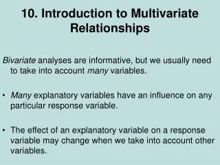
10. Introduction to Multivariate Relationships. Bivariate analyses are informative, but we usually need to take into account many variables. Many explanatory variables have an influence on any particular response variable.

10. Introduction to Multivariate Relationships
E N D
Presentation Transcript
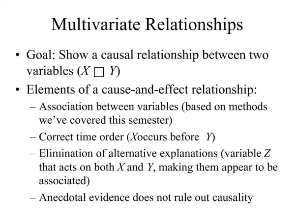
10. Introduction to Multivariate Relationships • Bivariate analyses are informative, but we usually need to take into account many variables. • Many explanatory variables have an influence on any particular response variable. • The effect of an explanatory variable on a response variable may change when we take into account other variables. Example (Ch.11, pp. 322-323): Florida county-wide data on x = education (% with at least a high school degree) and y = crime rate
Example: Y = whether admitted into grad school at U. California, Berkeley (for the 6 largest departments) X = gender Whether admitted Gender Yes No Total%yes Female 550 1285 1835 30% Male 1184 1507 2691 44% Difference of sample proportions = 0.44 – 0.30 = 0.14 has se = 0.014, Pearson 2 = 90.8 (df = 1),P-value = 0.00000…. There is very strong evidence of a higher probability of admission for men than for women.
Now let X1 = gender and X2 = department to which the person applied. e.g., for Department A, Whether admitted Gender Yes No Total%yes Female 89 19 108 82% Male 511 314 825 62% Now, 2 = 17.4 (df = 1), but difference is 0.62 – 0.82 = -0.20. The strong evidence is that there is a higher probability of being admitted for women than men. What happens with other departments?
Female Male Difference of Dept. Total %admittedTotal %admitted proportions 2 A 108 82% 825 62% -0.20 17.4 B 25 68% 560 63% -0.05 0.25 C 593 34% 325 37% 0.03 0.75 D 375 35% 417 33% -0.02 0.3 E 393 24% 191 28% 0.04 1.0 F 341 7% 273 6% -0.01 0.4 Total 1835 30% 2691 44% 0.14 90.8 There are 6 “partial tables,” which summed give the original “bivariate” table. How can the partial table results be so different from the bivariate table?
Partial tables – display association between two variables (Y and X1) at fixed levels of a “control variable” (X2). Example: Previous page shows results from partial tables relating Y = whether admitted to X1 = gender, controlling for (i.e., keeping constant) the level of X2= department. When a control variable X2 is kept constant, the association between Y and X1 is not due to the association of each of them with X2. Note: When each pair of variables is associated, then a bivariate association for two variables may differ from its partial association, controlling for the other variable.
Example: Y = whether admitted is associated with X1 = gender, but each of these itself associated with X2 = department. Department associated with gender: Males tend to apply more to departments A, B, females to C, D, E, F Department associated with whether admitted: % admitted higher for dept. A, B, lower for C, D, E, F Moral: Association does not imply causation! This is true for quantitative and categorical variables. e.g., a strong correlation between quantitative var’s X and Y does not mean that changes in X cause changes in Y.
Why does association not imply causation? • There may be some “alternative explanation” for the association. Example: Suppose there is a negative association between X = whether use marijuana regularly and Y = student GPA. Could the association be explained by some other variables that have an effect on each of these, such as achievement motivation or degree of interest in school or parental education? With observational data, effect of X on Y may be partly due to association of X and Y with lurking variables – variables that were not observed in the study but that influence the association of interest.
Causation difficult to assess with observational studies, unlike experimental studies that can control potential lurking variables (by randomization, keeping different groups “balanced” on other variables). In an observational study, when X1 and X2 both have effects on Y but are also associated with each other, there is said to be confounding. It’s difficult to determine whether either truly causes Y, because a variable’s effect could be partly due to its association with the other variable. (Example in Exercise 10.32 for X1 = amount of exercise, Y = number of serious illnesses in past year, X2 = age is a possible confounding variable)
Simpson’s paradox • It is possible for the (bivariate) association between two variables to be positive, yet be negative at each fixed level of a third variable. (see scatterplot) Example: Florida countywide data. There is a positive correlation between crime rate and education (% residents of county with at least a high school education)! There is a negative correlation between crime rate and education at each level of urbanization (% living in an urban environment) (see scatterplot)
Types of Multivariate Relationships • Spurious association: Y and X1 both depend on X2 and association disappears after controlling X2 (Karl Pearson 1897, one year after developing sample estimate of Galton’s correlation, now called “Pearson correlation”) Example: For nations, percent having home Internet connection negatively correlated with birth rate, but association disappears after control per capita gross domestic product (GDP).
Multiple causes – A variety of factors have influences on the response (most common in practice) In observational studies, usually all (or nearly all) explanatory variables have associations among themselves as well as with response var. Effect of any one changes depending on which other var’s are controlled (statistically), often because it has a direct effect and also indirect effects through other variables. Example: What causes Y = juvenile delinquency? X1 = Being from poor family? X2 = Being from a single-parent family? Perhaps X2 has a direct effect on Y and an indirect effect through its effect on X1.
Statistical interaction – Effect of X1on Y changes as the level of X2 changes. Example: Effect of whether a smoker (yes, no) on whether have lung cancer (yes, no) changes as value of age changes (essentially no effect for young people, stronger effect for old people) Example: U.S. median annual income by race and gender Race Gender Black White Female $25,700 $29,700 Male $30,900 $40,400
The difference in median income between whites and blacks is: $4000 for females, $9500 for males • i.e., the effect of race on income depends on gender (and the effect of gender on income depends on race), so there is interaction between race and gender in their effects on income. Example (p. 311):X = number of years of education Y = annualincome (1000’s of dollars) Suppose E(Y) = -10 + 4x for men E(Y) = - 5 + 2x for women The effect of education on income differs for men and women, so there is interaction between education and gender in their effects on income.
Some review questions • What does it mean to “control for a variable”? • When can we expect a bivariate association to change when we control for another variable? • Give an example of an association that you would expect to be spurious. • Draw a scatterplot showing a positive correlation for county-wide data on education and crime rate, but a negative association between those variables when we control for level of urbanization. • Why is it that association does not imply causation?