Download
1 / 20
200 likes | 239 Views
This term project aims to develop a methodology for mapping irrigation water requirements at a large-scale agricultural area, evaluate spatial variability and time-distribution of water requirements, and identify factors related to irrigated agricultural systems. The study area is a part of a large-scale irrigated area in Southern Italy, facing problems such as small land-holdings, market-oriented horticulture, rotation delivery schedule, and insufficient water distribution. The objective is to provide useful tools for irrigation managers to support decision-making processes. The methodology involves climate scenarios, climatic parameters, soil-water balance model, and GIS. The results include mapping of net irrigation requirements, aggregation at district level, and identification of errors and uncertainties in scaling up irrigation requirements.

E N D
“Determination of spatially-distributed irrigation water requirements at scheme level using soil-water balance model and GIS” Term Project – CEE 6440 – GIS in Water Resources Tuesday, November 30th 2004 Prepared by Daniel Zaccaria Graduate student Department of Irrigation Engineering Utah State University
OBJECTIVES General • Develop and test a tentative methodology for mapping I.W.R for large-scale agricultural areas, under different climatic scenarios • Evaluate spatial variability and time-distribution of I.W.R. along irrigation season Specific • Getting a better knowledge of main factors related to irrigated agricultural systems • Identifying major sources of errors and uncertainties in large-scale estimations of irrigation requirements
Long-term purposes • Carrying out preliminary studies in order to come up with a better irrigation water management plan for the study area • Carry out a performance analysis of distribution networks and eventually identify re-engineering options for low-performing systems or sub-systems OVERALL Show usefulness of coupling GIS environment and models capabilities to provide irrigation managers with operational tools to support decision-making processes
Background on the study area The study area is part of a large-scale irrigated area located in Southern Italy and managed by a local Water Users’ Association. The whole WUA scheme covers an area of 142,905 Ha
The study area is served by three large-scale irrigation schemes whose physical features and operational rules are different
Why this study area? Several problems • High number of small land-holdings (average farm size 1.5 -2.5 ha) • Market-oriented horticulture, which is strongly depending on irrigation • Irrigation networks are operated with rotation delivery schedule • Water distribution to farms is too restrictive and is not timely matching crop water requirements Resulting consequence • As a result of all the above factors, during the last 10 years a large number of farmers started developing their “private water sources” and refused to take water from large-scale irrigation networks. • This led to a very large number of unlicensed irrigation wells, to over-pumping from groundwater, to sea-water intrusion and salt accumulation in the soil ENVIRONMENTAL AND ECONOMIC HAZARDS
………. AND MOREOVER An alarming message is being continuously spread out: There is a serious water deficit in the area But before spreading such a message we have to be able to come up with reliable numbers from application of sound methodologies
Therefore: A good estimate of actual water demand is strongly needed at whole scheme level in order to identify: • Existence and potential magnitude of water deficit • Total volume of water seasonally withdrawn from groundwater • Existence and magnitude of environmental hazards • Re-engineering options (modernization and/or rehabilitation of irrigation systems) aiming at improving irrigation systems’ performances and efficiency of water use
Applied methodology 1st step) Identification of 3 climatic scenarios (Average, Demanding, Very-high demanding) 7 Climatic stations, monthly values for 35 years of observation (1959-1994) Areal Clim. Deficit = SUM [(ETo – Reff) x Station Weight] ETo computed on a montly basis by Hargreaves- Samani method ETo = 0.0023 Ra (Tmax – Tmin)0.5 (Ta + 17.8) Tmax and Tmin in hot-dry situation are quite different 35 annual values of Areal Climatic Deficit Probability of non-exceedance 50 %, 75 % and 90 Probabilities
Methodology Climatic parameters => Evapotranspiration (ETo) Crop Irrigation Requirements and their time-distribution depend on: Crop characteristics => Crop coefficient (Kc) Soil characteristics => WHC o AW (FC – PWP) Soil-Water Balance => accounting for all water inflows and outflows Di = D(i-1) + ETc – (P – SRO) – Iinf + DP - GW
Soils polygons (13 different soil types) + + Crops polygons (8 different crops) MeteoStations polygons + Intersect utility in ArcGIS
Identification of Simulation Units Simulation units are polygons having the same crop-soil-climatic area combinations 153 unique soil-crop-clim.area combinations = 153 ID.Codes (153 x 3 climatic scenarios) = 459 Runnings of the Soil-Water Balance model
Soil-Water Balance algorithm in terms of depletion Di = Di-1 + ETc - (P - SRO) - Irr + DP - GW • Assumptions: • irrigation aiming at maximum yield; 2) No groundwater contribution; 3) No restriction imposed • 4) Soils at F.C. at irrig. season starting Time to irrigate when: Di > MAD Wa Rz How much to irrigate? The amount necessary to replenish the root-zone to the F.C.
Superimposing layer of irrigation districts’ boundaries Aggregation of IWR at district level for different time-scales
Sources of errors and uncertainties in up-scaling IWR • Spatial variability of soils • Spatial variability of crops => different crop’s age and cultivars • Spatial variability of climatic conditions (Thiessen method enables rough estimation) • Spatial variability of land elevation (not taken into account) • Spatial variability of conveyance, distribution and application efficiencies Bottom line: I.W.R. are very close to what farmers give to crops in the area Further check the time-distribution of seasonal IWR values
Aknowledgements: • G. H. HARGREAVES • Stornara & Tara Water Users Association • Technical University of Lisbon (PT) – Instituto Superior de Agricultura QUESTIONS, COMMENTS OR SUGGESTIONS ??
Evaluating NIR and their spatial and time distribution Basic information for : • Water allocation plan • Water distribution plan (time of deliveries) • Indirect quantification of withdrawals from groundwater • Investigation on available water supply and time distribution • Comparing water supply with water demand enables identification of deficit periods and areas • Performance analysis of irrigation networks based on : • Water demand flow hydrographs • Physical capability of the network • Identify critical areas • Simulate re-engineering option and evaluating their effectiveness