Download
1 / 52
520 likes | 536 Views
Discover the impact of LANS-α turbulence model on resolution and energy transport in ocean modeling. Learn how LANS-α enhances realism and increases computational time.

E N D
The Lagrangian-Averaged Navier-Stokes alpha (LANS-) Turbulence Modelin Primitive Equation Ocean Modeling Mark R. Petersen with Matthew W. Hecht, Darryl D. Holm, and Beth A. Wingate Los Alamos National Laboratory Conclusion: LANS- produces turbulence statistics that resemble doubled-resolution simulations without LANS-. NCAR TOY Workshop February 26, 2008 LA-UR-05-0887
Rossby Radius of deformation Parallel Ocean Program (POP)Resolution is costly, but critical to the physics • Climate simulations • low resolution: 1 deg (100 km) • long duration: centuries • fully coupled to atmosphere, etc. • Eddy-resolving sim. • high resolution: 0.1 deg (10 km) • short duration: decades • ocean only Surface temperature 0.1º x 0.1º grid Surface temperature 1.0º x 1.0º grid
Scales resolved by global ocean models The Rossby Radius is the kinetic energy forcing scale. At the scale of the Rossby Radius, energy is converted from potential energy to kinetic energy. Satellite measurement data from Scott and Wang 2005
low resolution: 0.8º What do you get with higher resolution? cost of doubling horizontal grid is factor of 10 Small-scale turbulence and eddies transport energy and heat. Reynolds decomposition: 0.4º perturbation total time average 0.2º • These become more realistic • with higher resolution: • eddy heat transport: • eddy kinetic energy: • feedback of small-scale features on the large-scale mean flow - important for oceanic jets • vertical temperature profile high resolution: 0.1º note: SST and thus heat flux is main influence on atmosphere for climate
Lagrangian-Averaged Navier-Stokes Equation (LANS-) rough smooth larger smooths more Lagrangian averaged velocity u Eulerian averaged velocity rough smooth Helmholtz operator advection extra nonlinear term Coriolis pressure gradient diffusion
The test problem: Idealization of Antarctic Circumpolar Current up solid boundary N 12ºC surface thermal forcing periodic bndry zonal wind E periodic bndry 2ºC solid boundary deep-sea ridge This test problem invokes the baroclinic instability.
Kinetic energy high res low res resolution: 0.8° 0.4° 0.2° 0.1° Eddy kinetic energy high res low res resolution: 0.8° 0.4° 0.2° 0.1° Depth of 6C isotherm 0.1° (high res) 0.2° 0.4° 0.8° (low res) Test problem results, POP only Surface temperature low resolution-0.8º standard POP high resolution-0.1º standard POP Potential temperature - vertical cross section warm surf. forcing warm surf. forcing depth depth low resolution-0.8º standard POP high resolution-0.1º standard POP S N S N
POP- with Helmholtz inversion: vary alpha… POP- with filters: vary the filter width… Kinetic energy Kinetic energy filter width Eddy kinetic energy Eddy kinetic energy
Test Problem Results: Baroclinic Instability 6C isotherm Vertical temperature profile 0.1°(high res) 0.2° 0.4° 0.8°(low res) 0.2° 0.1° 0.4° 0.8°(low res)
Test Problem Results: Baroclinic Instability 6C isotherm Vertical temperature profile 0.1°(high res) 0.2° POP- 0.2° 0.4° POP- 0.4° 0.8° POP- 0.8°(low res) 0.2° 0.1° 0.4° 0.8°(low res) 0.2° POP- 0.4° POP- 0.8° POP-
How does the Leray model compare to LANS-alpha? extra nonlinear term not in Leray model Vertical temperature profile Leray produces similar results as LANS-alpha, but to a lesser degree.
Dispersion Relation for LANS-using linearized shallow water equations Gravity waves Rossby waves normally: normally: with LANS-: LANS-: frequency , wavenumber k, gravity g, height H Rossby radius beta Dispersion relation Dispersion relation normal with LANS- normal with LANS- LANS- slows down gravity and Rossby waves at high wave number.
What does LANS- do to the Rossby Radius? Solve for kR, the wavenumber of the Rossby Radius: Use that to find R*, the effective Rossby Radius, as a function of : kR Dispersion relation * kR normal LANS-, small LANS-, larger LANS- makes the Rossby Radius effectively larger.
Adding LANS- increases computation time by <30% We can take larger timesteps with LANS-
POP-alpha in the North Atlantic • POP- is still under development for realistic domains. • Rough topography and high velocities in jets cause difficulties. • The Leray model, a simplified version of LANS-, shows promising results: higher kinetic and eddy kinetic energy. POP-Leray 0.2º Eddy kinetic energy (3yr mean) kinetic energy Smith ea 200 p 1550 0.1 mKE: 13.2 total KE=~43 smooth u^2: 9.7 global avg
cross section through North Atlantic current POP 0.2º EKE POP-Leray 0.2º EKE POP 0.1º EKE POP-alpha in the North Atlantic POP 0.2º EKE POP-Leray 0.2º EKE POP 0.1º EKE
Conclusions • LANS- produces turbulence statistics that resemble doubled-resolution simulations without LANS- in: • Kinetic energy • Eddy kinetic energy • Temperature distributions associate with baroclinic instability • LANS- increases computation time by 30%, as opposed to a factor of 8-10 to double the resolution. • Current work: simulations using LANS-alpha in realistic domains, such as the North Atlantic domain.
Can you see more eddies with LANS-alpha? POP, 0.4º resolution POP, 0.2º resolution POP-, 0.4º resolution Pot. Temperature Pot. Temperature Pot. Temperature Velocity Velocity Velocity All sections at a depth of 1600m rough velocity: red, smooth: black
How should we measure kinetic energy with LANS-alpha? Kinetic Energy Eddy Kinetic Energy
What are my boundary conditions? Option 1: shrink filter at boundary Option 2: shrink filter near boundary Option 3: make filter weights=0 on land water land water land water land
A Possibility: Use variable alpha We are thinking about this…
Parallel Ocean Program (POP) Resolution: 0.1° global. Color shows speed.
Outline • Resolution of eddies in ocean simulations • LANS- implementation in POP • Idealized test case: the channel domain • The real thing: the North Atlantic
hydrostatic in the vertical equation of state Parallel Ocean Program (POP) conservation of momentum u hor. velocity w vertical velocity tracer t time p pressure 0 density T temperature S salinity • Bryan-Cox type model, z-level vertical grid, finite difference model diffusion advection Coriolis pressure gradient conservation of mass for incompressible fluid grid conservation of tracers (temperature, salinity) source/ sink diffusion advection
Outline • Resolution of eddies in ocean simulations • LANS- implementation in POP • Idealized test case: the channel domain • The real thing: the North Atlantic
The POP-alpha model Issue #1: How do we implement the alpha model within the barotropic/baroclinic splitting of POP? level 1 level 2 level 3 level K full ocean (vertical section) fast surface gravity waves level 1 level 2 level 3 level K slower internal gravity waves vertically integrated • barotropic part • single layer • implicit time step • baroclinic part • multiple levels • explicit time step • vertical mean = 0
Barotropic Algorithm - Pop-alpha Simultaneously solve for: free surface height and both velocities, Invert using iterative CG routine smoothing within each iteration is too costly! momentum forcing terms momentum forcing terms resolution:
Barotropic Algorithm - Pop-alpha Simultaneously solve for: free surface height and both velocities, Invert using iterative CG routine smoothing within each iteration is too costly! What if we eliminate just this one smoothing step? momentum forcing terms momentum forcing terms resolution:
The POP-alpha model Issue #2: How should we compute the smooth velocity u? Helmholtz inversion is costly! Common to use a filter instead: filter width 3 • Wider filters result in: • Stronger smoothing • Effects are like larger • More computation • More ghostcells filter width 5 filter width 7 filter width 9
Outline • Resolution of eddies in ocean simulations • LANS- implementation in POP • Idealized test case: the channel domain • The real thing: the North Atlantic
Outline • Resolution of eddies in ocean simulations • LANS- implementation in POP • Idealized test case: the channel domain • The real thing: the North Atlantic
Homo sapiens neanderthalensis currently: 380 ppm Homo sapiens archaic Homo sapiens sapiens Homo erectus CO2 ice core record domesticated plants & animals Siegenthaler et.al. Science 2005
Community Climate System Model • Collaboration of: • National Center for Atmospheric Research (NCAR) in Boulder, CO • Los Alamos National Laboratory (LANL) Atmosphere (NCAR) Land Surface (NCAR) Flux Coupler Ocean POP (LANL) Sea Ice (LANL)
Main activity: Assessment reports • Third Assessment Report: 2001 • Fourth Assessment Report: 2007 • Fifth: planned for 2013 IPCC - Intergovernmental Panel on Climate Change • Created in 1988 by World Meteorological Organization (WMO) and United Nations Environment Programme (UNEP) • Role of IPCC: assess on a comprehensive, objective, open and transparent basis the scientific, technical and socio-economic information relevant to understanding: • the scientific basis of risk of human-induced climate change • its potential impacts and • options for adaptation and mitigation.
IPCC scenarios of future emissions economic models carbon cycle models IS92a: business as usual (extrapolation from current rates of increase)
scenarios CO2 concentration ensemble of climate models average of ensemble Temperature change scenario A2 Final product CO2 emissions economic models carbon cycle models
IPCC: Estimates of confidence TAR p.82
Standard POP tracer equation diffusion advection momentum equation diffusion advection e.g. centrifugal pressure gradient Coriolis POP-alpha rough velocity, smooth velocity, tracer equation diffusion advection momentum equation diffusion advection extra nonlinear term Coriolis e.g. centrifugal pressure gradient Helmholtz inversion
Outline • POP ocean model & climate change assessment • LANS- implementation in POP • Idealized test case: the channel domain • The real thing: the North Atlantic
The POP-alpha model Issues: How do we smooth the velocity in an Ocean General Circulation Model? rough smooth or: use a filter Helmholtz inversion for example, a top-hat filter is costly!
1 -1 1 -1 1 -1 Filter Instabilities 1D filter, If , smoothing filters out the Nyquist frequency. rough gridpoints smooth The smooth velocity is blind to this oscillation. Therefore, the free surface height cannot counter it!
Filter Instabilities 1D filter, If , smoothing filters out the Nyquist frequency. rough 370 m/s smooth 30 m/s Condition for stability is
Filter: Conditions for stability rough velocity filter:
Filter analysis: Helmholtz inversion Green’s function Then compute Take v to be a point source: Can use this to understand filter near boundaries:
Temperature - hor. mean high res POP med. res POP Filters • Wider filters result in: • Stronger smoothing • Effects are like larger • More computation • More ghostcells filter width 3 filter width 5 filter width 7 filter width 9
Filters • Wider filters result in: • Stronger smoothing • Effects are like larger • More computation • More ghostcells filter width 3 filter width 5 Temperature - hor. mean high res POP filter width 7 med. res POP filter width 9 width 9 width 7 width 5 width 3 med. res POP-
What are my boundary conditions? Option 1: shrink filter at boundary Option 2: shrink filter near boundary Option 3: make filter weights=0 on land water land water land water land
A Possibility: Use variable alpha We are thinking about this…