Efficient Quantitative Frequent Pattern Mining Using Predicate Trees
Explore Predicate tree approach for quantitative frequent pattern mining. Learn about P-trees, advantages of PQM, and construction methods. Enhance your understanding of Predicate value P-trees and range trees. Optimize performance with this detailed analysis.

Efficient Quantitative Frequent Pattern Mining Using Predicate Trees
E N D
Presentation Transcript
Efficient Quantitative Frequent Pattern Mining Using Predicate Trees Baoying Wang, Fei Pan, Yue Cui William Perrizo North Dakota State University
Outline • Introduction • Review of Predicate trees • Quantitative frequent pattern mining • Performance analysis • Summary
Introduction • ARM was first introduced by Agrawal et al in 1993. • ARM can be used for categorical and quantitative attributes. • The approach of categorical ARM is extended to the quantitative data by using intervals. • An example would be: age[30,45] and income[40, 60] #car[1, 2].
Limitations of Traditional Tree Structures • Tree structures used in quantitative ARM: hash trees, R-trees, prefix-trees, FP-trees, etc. • They are built on-the-fly according to the chosen quantitative intervals. • There is need to rebuild these trees when intervals change
Predicate Tree Approach • In this paper, we present Predicate tree based quantitative frequent pattern mining (PQM). • The central idea of PQM is to exploit predicate P-trees to get frequent pattern counts of any quantitative interval. • Predicate-trees (P-trees) are lossless, vertical bitwise compressed data structures.
Advantages of PQM • P-trees are pre-generated tree structures, which are flexible and efficient for any data partition and interval optimization; • PQM is efficient by using fast P-tree logic operations; • PQM has better support threshold scalability and cardinality scalability due to the vertically decomposed structure and compression of P-trees.
Outline • Introduction • Review of Predicate trees • Quantitative frequent pattern mining • Performance analysis • Summary
Review Of Predicate Trees • A Predicate tree (P-tree) is a lossless, vertical bitwise compressed data structure. • A P-tree can be 1-dimensional, 2-dimensional, 3-dimensional, etc. • In this paper, we focus on 1-dimensional P-trees.
Construction of P-trees • Given a data set with d attributes, R = (A1, A2 … Ad), and the binary representation of jth attribute Aj as bj,mbj,m-1...bj,i… bj,1. • To build up a 1-D P-tree: • Attributes are decomposed into bit files, one file for each bit position; • A bit file is recursively partitioned into halves and each half into sub-halves until the sub-half is pure (entirely 1-bits or entirely 0-bits).
Horizontal structure Processed vertically (scans) 0 0 0 0 1 0 1 1 0 0 0 1 0 01 0 1 0 1 0 0 1 0 0 1 01 1. Whole file is not pure1 0 2. 1st half is not pure1 0 0 0 0 0 1 01 3. 2nd half is not pure1 0 0 0 0 0 1 0 0 10 01 0 0 0 1 0 0 0 0 0 0 0 1 01 10 0 0 0 0 1 10 0 0 0 0 1 0 0 0 0 0 0 0 1 1 0 0 0 0 0 0 0 0 0 0 1 10 0 1 0 0 0 0 1 0 1 4. 1st half of 2nd half not 0 0 0 1 0 1 01 5. 2nd half of 2nd half is 1 0 1 0 6. 1st half of 1st of 2nd is 1 7. 2nd half of 1st of 2nd not 0 Construction of P-trees(Cont.) --> R[A1] R[A2] R[A3] R[A4] R(A1 A2 A3 A4) 010 111 110 001 011 111 110 000 010 110 101 001 010 111 101 111 101 010 001 100 010 010 001 101 111 000 001 100 111 000 001 100 010 111 110 001 011 111 110 000 010 110 101 001 010 111 101 111 101 010 001 100 010 010 001 101 111 000 001 100 111 000 001 100 R11 R12 R13 R21 R22 R23 R31 R32 R33 R41 R42 R43 0 1 0 1 1 1 1 1 0 0 0 1 0 1 1 1 1 1 1 1 0 0 0 0 0 1 0 1 1 0 1 0 1 0 0 1 0 1 0 1 1 1 1 0 1 1 1 1 1 0 1 0 1 0 0 0 1 1 0 0 0 1 0 0 1 0 0 0 1 1 0 1 1 1 1 0 0 0 0 0 1 1 0 0 1 1 1 0 0 0 0 0 1 1 0 0 P11 P12 P13 P21 P22 P23 P31 P32 P33 P41 P42 P43
Pure1 trees and logical operations 0 0 0 • Pure1 trees: • Operations: 0 0 0 1 0 0 0 0 0 0 1 1 0 1 1 0 0 1 0 1 1 0 P11 P12 P13 0 0 0 0 0 0 0 0 0 0 0 0 0 1 0 1 1 0 0 1 0 0 1 0 1 1 0 P11P12 P11 P13 P13’
Predicate value P-tree: Px=v • A value P-tree represents a tuple subset, X, of all tuples containing a specified value, v, of an attribute, A. It is denoted by PA,v • Let v=bmbm-1…b1, where bi is ith bit of v in binary. There are two steps to calculate Pv. • 1) Get the bit-value-Ptree PA,v,i for each bit position of v according to the bit value: If bi = 1, PA,v,i = Pi;Otherwise PA,v,i = Pi’, • 2) Calculate PA,v by ANDing all the bit-value-Ptrees of v, i.e. PA,v = Pbm Pbm-1… Pb1
Predicate range tree: Pxv • v=bm…bi…b1 • Pxv = P’m opm … P’i opi P’i-1 … opk+1P’k 1) opi is if bi=0, opi is otherwise 2) k is the rightmost bit position with value of “0” 3) the operators are right binding. • For example: Px 101 = (P’2 P’1)
Predicate range tree: Pxv • v=bm…bi…b1 • Pxv = Pm opm … Pi opi Pi-1 … opk+1 Pk 1) opi is if bi=1, opi is otherwise 2) k is the rightmost bit position with value of “0” 3) the operators are right binding. • For example: Px 101 = (P2 (P1 P0))
Outline • Introduction • Review of Predicate trees • Quantitative frequent pattern mining • Performance analysis • Summary
P-tree Quantitative Frequent Pattern Mining (PQM) • The central idea of PQM is to exploit P-trees to get frequent pattern counts of any quantitative interval. • P-trees, unlike other tree structures, are pre-generated. There is no need to construct trees on-the-fly during interval generations and merges. • Interval P-tree: PlAu = PAl PAu • PAl and PAu are predicate range trees for predicates Al and Au
PQM algorithm • Determine the number of partitions for each quantitative attribute; • Calculate support of each 1-item pattern using Predicate trees. For quantitative attributes, adjacent intervals are combined if their support is below the user-defined threshold; • Select patterns with minimum support to get frequent patterns; • Generate (k+1)-item frequent pattern candidates based on k-item frequent patterns; • Calculate support of each (k+1)-item frequent pattern candidates.
Example of PQM (Cont.) • Interval: age [30, 45]10 or age [011110, 101101]2 • P30age45 = Page30 Page45 = Page011110 Page101101. • Root count of P30age45,Nage30,45, denotes the number of transactions that involves age[30, 45].
When the interval changes • Use the same P-trees and only need to calculate range P-trees based on the new boundary values. • Especially when two adjacent intervals are merged, there is no need to calculate the new range P-trees from the scratch. • We can simply OR two range P-trees for two adjacent intervals. • Example: P15age45 = P15age29 P30age45
Multi-item pattern mining • AND the P-tree of each item pattern to get the multi-item pattern P-tree • The item can be categorical or quantitative. • Example: we want to find 2-item pattern age[30,45] and sex = 1 • 2-item pattern P-tree P30age45, sex=1 = P30age45 AND Psex=1
Outline • Introduction • Review of Predicate trees • Quantitative frequent pattern mining • Performance analysis • Summary
Run Time (s) 700 PQM 600 500 Apriori 400 300 200 100 0% 20% 40% 60% 80% 100% Support threshold Performance Analysis The experiment results show PQM algorithm is more scalable than Apriori in terms of support threshold and the number of transactions. a) Scalability with support threshold b) Scalability with transaction size
Summary • In this paper, we present a quantitative frequent pattern mining algorithm using P-trees (PQM). • P-trees can be used for any interval. There is no need to build P-trees on-the-fly. • P-trees are not only flexible but also efficient for interval optimization. • Fast P-tree logic operations are used to achieve efficient frequent pattern mining. • Our approach has better performance due to the vertical decomposed data structure and compression of P-trees