Model selection
Model selection. Stepwise regression. Statement of problem. A common problem is that there is a large set of candidate predictor variables. (Note: The examples herein are really not that large.)


Model selection
E N D
Presentation Transcript
Model selection Stepwise regression
Statement of problem • A common problem is that there is a large set of candidate predictor variables. • (Note: The examples herein are really not that large.) • Goal is to choose a small subset from the larger set so that the resulting regression model is simple, yet have good predictive ability.
Example: Cement data • Response y: heat evolved in calories during hardening of cement on a per gram basis • Predictor x1: % of tricalcium aluminate • Predictor x2: % of tricalcium silicate • Predictor x3: % of tetracalcium alumino ferrite • Predictor x4: % of dicalcium silicate
Two basic methods of selecting predictors • Stepwise regression: Enter and remove predictors, in a stepwise manner, until there is no justifiable reason to enter or remove more. • Best subsets regression: Select the subset of predictors that do the best at meeting some well-defined objective criterion.
Stepwise regression: the idea • Start with no predictors in the “stepwise model.” • At each step, enter or remove a predictor based on partial F-tests (that is, the t-tests). • Stop when no more predictors can be justifiably entered or removed from the stepwise model.
Stepwise regression: Preliminary steps • Specify an Alpha-to-Enter (αE = 0.15) significance level. • Specify an Alpha-to-Remove (αR = 0.15) significance level.
Stepwise regression: Step #1 • Fit each of the one-predictor models, that is, regress y on x1, regress y on x2, … regress y on xp-1. • The first predictor put in the stepwise model is the predictor that has the smallest t-test P-value (below αE = 0.15). • If no P-value < 0.15, stop.
Stepwise regression:Step #2 • Suppose x1 was the “best” one predictor. • Fit each of the two-predictor models with x1 in the model, that is, regress y on (x1, x2), regress y on (x1, x3), …, and y on (x1, xp-1). • The second predictor put in stepwise model is the predictor that has the smallest t-test P-value (below αE = 0.15). • If no P-value < 0.15, stop.
Stepwise regression:Step #2 (continued) • Suppose x2 was the “best” second predictor. • Step back and check P-value for β1 = 0. If the P-value for β1 = 0 has become not significant (above αR = 0.15), remove x1 from the stepwise model.
Stepwise regression:Step #3 • Suppose both x1 and x2 made it into the two-predictor stepwise model. • Fit each of the three-predictor models with x1 and x2 in the model, that is, regress y on (x1, x2, x3), regress y on (x1, x2, x4), …, and regress y on (x1, x2, xp-1).
Stepwise regression:Step #3 (continued) • The third predictor put in stepwise model is the predictor that has the smallest t-test P-value (below αE = 0.15). • If no P-value < 0.15, stop. • Step back and check P-values for β1 = 0 andβ2 = 0. If either P-value has become not significant (above αR = 0.15), remove the predictorfrom the stepwise model.
Stepwise regression:Stopping the procedure • The procedure is stopped when adding an additional predictor does not yield a t-test P-value below αE = 0.15.
Predictor Coef SE Coef T P Constant 81.479 4.927 16.54 0.000 x1 1.8687 0.5264 3.55 0.005 Predictor Coef SE Coef T P Constant 57.424 8.491 6.76 0.000 x2 0.7891 0.1684 4.69 0.001 Predictor Coef SE Coef T P Constant 110.203 7.948 13.87 0.000 x3 -1.2558 0.5984 -2.10 0.060 Predictor Coef SE Coef T P Constant 117.568 5.262 22.34 0.000 x4 -0.7382 0.1546 -4.77 0.001
Predictor Coef SE Coef T P Constant 103.097 2.124 48.54 0.000 x4 -0.61395 0.04864 -12.62 0.000 x1 1.4400 0.1384 10.40 0.000 Predictor Coef SE Coef T P Constant 94.16 56.63 1.66 0.127 x4 -0.4569 0.6960 -0.66 0.526 x2 0.3109 0.7486 0.42 0.687 Predictor Coef SE Coef T P Constant 131.282 3.275 40.09 0.000 x4 -0.72460 0.07233 -10.02 0.000 x3 -1.1999 0.1890 -6.35 0.000
Predictor Coef SE Coef T P Constant 71.65 14.14 5.07 0.001 x4 -0.2365 0.1733 -1.37 0.205 x1 1.4519 0.1170 12.41 0.000 x2 0.4161 0.1856 2.24 0.052 Predictor Coef SE Coef T P Constant 111.684 4.562 24.48 0.000 x4 -0.64280 0.04454 -14.43 0.000 x1 1.0519 0.2237 4.70 0.001 x3 -0.4100 0.1992 -2.06 0.070
Predictor Coef SE Coef T P Constant 52.577 2.286 23.00 0.000 x1 1.4683 0.1213 12.10 0.000 x2 0.66225 0.04585 14.44 0.000
Predictor Coef SE Coef T P Constant 71.65 14.14 5.07 0.001 x1 1.4519 0.1170 12.41 0.000 x2 0.4161 0.1856 2.24 0.052 x4 -0.2365 0.1733 -1.37 0.205 Predictor Coef SE Coef T P Constant 48.194 3.913 12.32 0.000 x1 1.6959 0.2046 8.29 0.000 x2 0.65691 0.04423 14.85 0.000 x3 0.2500 0.1847 1.35 0.209
Predictor Coef SE Coef T P Constant 52.577 2.286 23.00 0.000 x1 1.4683 0.1213 12.10 0.000 x2 0.66225 0.04585 14.44 0.000
Stepwise Regression: y versus x1, x2, x3, x4 Alpha-to-Enter: 0.15 Alpha-to-Remove: 0.15 Response is y on 4 predictors, with N = 13 Step 1 2 3 4 Constant 117.57 103.10 71.65 52.58 x4 -0.738 -0.614 -0.237 T-Value -4.77 -12.62 -1.37 P-Value 0.001 0.000 0.205 x1 1.44 1.45 1.47 T-Value 10.40 12.41 12.10 P-Value 0.000 0.000 0.000 x2 0.416 0.662 T-Value 2.24 14.44 P-Value 0.052 0.000 S 8.96 2.73 2.31 2.41 R-Sq 67.45 97.25 98.23 97.87 R-Sq(adj) 64.50 96.70 97.64 97.44 C-p 138.7 5.5 3.0 2.7
Caution about stepwise regression! • Do not jump to the conclusion … • that all the important predictor variables for predicting y have been identified, or • that all the unimportant predictor variables have been eliminated.
Caution about stepwise regression! • Many t-tests for βk= 0are conducted in a stepwise regression procedure. • The probability is high … • that we included some unimportant predictors • that we excluded some important predictors
Drawbacks of stepwise regression • The final model is not guaranteed to be optimal in any specified sense. • The procedure yields a single final model, although in practice there are often several equally good models. • It doesn’t take into account a researcher’s knowledge about the predictors.
Stepwise Regression: PIQ versus MRI, Height, Weight Alpha-to-Enter: 0.15 Alpha-to-Remove: 0.15 Response is PIQ on 3 predictors, with N = 38 Step 1 2 Constant 4.652 111.276 MRI 1.18 2.06 T-Value 2.45 3.77 P-Value 0.019 0.001 Height -2.73 T-Value -2.75 P-Value 0.009 S 21.2 19.5 R-Sq 14.27 29.49 R-Sq(adj) 11.89 25.46 C-p 7.3 2.0
The regression equation is PIQ = 111 + 2.06 MRI - 2.73 Height Predictor Coef SE Coef T P Constant 111.28 55.87 1.99 0.054 MRI 2.0606 0.5466 3.77 0.001 Height -2.7299 0.9932 -2.75 0.009 S = 19.51 R-Sq = 29.5% R-Sq(adj) = 25.5% Analysis of Variance Source DF SS MS F P Regression 2 5572.7 2786.4 7.32 0.002 Error 35 13321.8 380.6 Total 37 18894.6 Source DF Seq SS MRI 1 2697.1 Height 1 2875.6
Stepwise Regression: BP versus Age, Weight, BSA, Duration, Pulse, Stress Alpha-to-Enter: 0.15 Alpha-to-Remove: 0.15 Response is BP on 6 predictors, with N = 20 Step 1 2 3 Constant 2.205 -16.579 -13.667 Weight 1.201 1.033 0.906 T-Value 12.92 33.15 18.49 P-Value 0.000 0.000 0.000 Age 0.708 0.702 T-Value 13.23 15.96 P-Value 0.000 0.000 BSA 4.6 T-Value 3.04 P-Value 0.008 S 1.74 0.533 0.437 R-Sq 90.26 99.14 99.45 R-Sq(adj) 89.72 99.04 99.35 C-p 312.8 15.1 6.4
The regression equation is BP = - 13.7 + 0.702 Age + 0.906 Weight + 4.63 BSA Predictor Coef SE Coef T P Constant -13.667 2.647 -5.16 0.000 Age 0.70162 0.04396 15.96 0.000 Weight 0.90582 0.04899 18.49 0.000 BSA 4.627 1.521 3.04 0.008 S = 0.4370 R-Sq = 99.5% R-Sq(adj) = 99.4% Analysis of Variance Source DF SS MS F P Regression 3 556.94 185.65 971.93 0.000 Error 16 3.06 0.19 Total 19 560.00 Source DF Seq SS Age 1 243.27 Weight 1 311.91 BSA 1 1.77
Stepwise regression in Minitab • Stat >> Regression >> Stepwise … • Specify response and all possible predictors. • If desired, specify predictors that must be included in every model. (This is where researcher’s knowledge helps!!) • Select OK. Results appear in session window.