Fixed-point design
Fixed-point design. SYSC5603 (ELG6163) Digital Signal Processing Microprocessors, Software and Applications Miodrag Bolic. Overview. Introduction Numeric representation Simulation methods for floating to fixed point conversion Analytical methods. Fixed-Point Design.

Fixed-point design
E N D
Presentation Transcript
Fixed-point design SYSC5603 (ELG6163) Digital Signal Processing Microprocessors, Software and Applications Miodrag Bolic
Overview • Introduction • Numeric representation • Simulation methods for floating to fixed point conversion • Analytical methods
Fixed-Point Design • Digital signal processing algorithms • Often developed in floating point • Later mapped into fixed point for digital hardware realization • Fixed-point digital hardware • Lower area • Lower power • Lower per unit production cost Copyright Kyungtae Han [2]
Fixed-Point Design • Float-to-fixed point conversion required to target • ASIC and fixed-point digital signal processor core • FPGA and fixed-point microprocessor core • All variables have to be annotated manually • Avoid overflow • Minimize quantization effects • Find optimum wordlength • Manual process supported by simulation • Time-consuming • Error prone Copyright Kyungtae Han [2]
Wordlength S X X X X X Wordlength Integer wordlength X X X X X Integer wordlength = 2 Fixed-Point Representation • Fixed point type • Wordlength • Integer wordlength • Quantization modes • Round • Truncation • Overflow modes • Saturation • Saturation to zero • Wrap-around SystemC format www.systemc.org Back Copyright Kyungtae Han [2]
Tools for Fixed-Point Simulation • gFix (Seoul National University) • Using C++, operator overloading • Simulink (Mathworks) • Fixed-point block set 4.0 • SPW (Cadence) • Hardware design system • CoCentric (Synopsys) • Fixed-point designer float a; float b; float c; c = a + b; gFix a(12,1); gFix b(12,1); gFix c(13,2); c = a + b; • Wordlengths determined manually • Wordlength optimization tool needed Copyright Kyungtae Han [2]
Optimum Wordlength • Longer wordlength • May improve applicationperformance • Increases hardware cost • Shorter wordlength • May increase quantization errorsand overflows • Reduces hardware cost • Optimum wordlength • Maximize application performanceor minimize quantization error • Minimize hardware cost Optimum wordlength Distortion d(w) [1/performance] Cost c(w) Wordlength (w) Copyright Kyungtae Han [2]
Wordlength Optimization Approach • Analytical approach • Quantization error model • For feedback systems, instability and limit cycles can occur • Difficult to develop analytical quantization error model of adaptive or non-linear systems • Simulation-based approach • Wordlengths chosen while observing error criteria • Repeated until wordlengths converge • Long simulation time Copyright Kyungtae Han [2]
Overview • Introduction • Numeric representation • Simulation methods for floating to fixed point conversion • Analytical methods
Number representation Matlab examples • Numeric circle • fi Basics • fi Binary Point Scaling
Fi type www.mathworks.com
Fi object www.mathworks.com
Fi Object • Notation • Multiplication • Multiplication with KeepMSB Mode • Addition • Addition with KeepLsb Mode • Numerictype • fimath www.mathworks.com
Overview • Introduction • Numeric representation • Simulation methods for floating to fixed point conversion • Analytical methods
Data-range propagation y1=2.1x1-1.8(x1+x2)=0.3x1-1.8x2 Input range: (-0.6 0.6) Output range: (-1.26, 1.26) [Constantinides04]
Data-range propagation Disadvantages • Provide larger bounds on signal values than necessary Solution • Simulation-based range estimation
Development of fixed point programs • Toolbox gFix [Sung95]
Implementation – range estimation [Sung95]
Implementation – range estimation [Sung95]
Result of the range estimator [Sung95]
Fixed point simulation [Sung95]
Operator overloading [Sung95]
Fixed-precision algorithm [Sung95]
Reducing the number of overflows in Matlab 1. Implement textbook algorithm in M. 2. Verify with builtin floating-point in M. 3. Convert to fixed-point in M and run with default settings. 4. Override the fi object with 'double' data type to log min and max values. 5. Use logged min and max values to set the fixed-point scaling. 6. Validate the fixed-point solution. 7. Convert M to C using Embedded MATLAB or Simulink to FPGA using Altera and Xilinx tools. www.mathworks.com
Matlab functions • logreport • fi_best_numeric_type_from_logs
Overview • Introduction • Numeric representation • Simulation methods for floating to fixed point conversion • Analytical methods
Filter Implementation • Finite word-length effects (fixed point implementation) - Coefficient quantization - Overflow & quantization in arithmetic operations - scaling to prevent overflow - quantization noise statistical modeling - limit cycle oscillations CopyrightMarc Moonen [1]
Coefficient Quantization The coefficient quantization problem : • Filter design in Matlab (e.g.) provides filter coefficients to 15 decimal digits (such that filter meets specifications) • For implementation, need to quantize coefficients to the word length used for the implementation. • As a result, implemented filter may fail to meet specifications… ?? • PS: In present-day signal processors, this has become less of a problem (e.g. with 16 bits (=4 decimal digits) or 24 bits (=7 decimal digits) precision). In hardware design, with tight speed requirements, this is still a relevant problem. CopyrightMarc Moonen [1]
Coefficient Quantization Coefficient quantization effect on pole locations : -> tightly spaced poles (e.g. for narrow band filters) imply high sensitivity of pole locations to coefficient quantization -> hence preference for low-order systems (parallel/cascade) Example: Implementation of a band-pass IIR 12-order filter Direct form with 16-bit coeff. Cascade structure with 16-bit coeff.
Coefficient Quantization Coefficient quantization effect on pole locations : • example : 2nd-order system (e.g. for cascade realization) CopyrightMarc Moonen [1]
Coefficient Quantization • example (continued) : with 5 bits per coefficient, all possible pole positions are... Low density of permissible pole locations at z=1, z=-1, hence problem for narrow-band LP and HP filters CopyrightMarc Moonen [1]
u[k] + + + - y[k] Coefficient Quantization • example (continued) : possible remedy: `coupled realization’ poles are where are realized/quantized hence permissible pole locations are (5 bits) CopyrightMarc Moonen [1]
Quantization of an FIR filter • Transfer function ΔH(z) • The effect of coefficient quantization to linear phase [Oppenheim98]
FIR filter example • Passband attenuation 0.01, Radial frequency (0,0.4) • Stopband attenuation 0.001, Radial frequency (0.4, ) [Oppenheim98]
FIR filter example – 16bits [Oppenheim98]
FIR filter example - 8bits [Oppenheim98]
Arithmetic Operations Finite word-length effects in arithmetic operations: • Inlinear filters, have to consider additions & multiplications • Addition: if, two B-bit numbers are added, the result has (B+1) bits. • Multiplication: if a B1-bit number is multiplied by a B2-bit number, the result has (B1+B2-1) bits. For instance, two B-bit numbers yield a (2B-1)-bit product • Typically (especially so in an IIR (feedback) filter), the result of an addition/multiplication has to be represented again as a B’-bit number (e.g. B’=B). Hence have to get rid of either most significant bits or least significant bits… CopyrightMarc Moonen [1]
Arithmetic Operations • Option-1: Most significant bits If the result is known to be upper bounded so that the most significant bit(s) is(are) always redundant, it(they) can be dropped, without loss of accuracy. This implies we have to monitor potential overflow, and introduce scaling strategyto avoid overflow. • Option-2 : Least significant bits Rounding/truncation/… to B’ bits introduces quantization noise. The effect of quantization noise is usually analyzed in a statistical manner. Quantization, however, is a deterministic non-linear effect, which may give rise to limit cycle oscillations. CopyrightMarc Moonen [1]
Scaling The scaling problem: • Finite word-length implementation implies maximum representable number. Whenever a signal (output or internal) exceeds this value, overflow occurs. • Digital overflow may lead (e.g. in 2’s-complement arithmetic) to polarity reversal (instead of saturation such as in analog circuits), hence may be very harmful. • Avoid overflow through proper signal scaling • Scaled transfer function may be c*H(z) instead of H(z) (hence need proper tracing of scaling factors) CopyrightMarc Moonen [1]
Scaling Time domain scaling: • Assume input signal is bounded in magnitude (i.e. u-max is the largest number that can be represented in the `words’ reserved for the input signal’) • Then output signal is bounded by • To satisfy (i.e. y-max is the largest number that can be represented in the `words’ reserved for the output signal’) we have to scale H(z) to c.H(z), with CopyrightMarc Moonen [1]
Scaling • Example: • assume u[k] comes from 12-bit A/D-converter • assume we use 16-bit arithmetic for y[k] & multiplier • hence inputs u[k] have to be shifted by 3 bits to the right before entering the filter (=loss of accuracy!) u[k] + 0.99 x y[k] + shift u[k] 0.99 x y[k] CopyrightMarc Moonen [1]
Scaling L2-scaling: (`scaling in L2 sense’) • Time-domain scaling is simple & guarantees that overflow will never occur, but often over-conservative (=too small c) • If an `energy upper bound’ for the input signal is known then L2-scaling uses where …is an L2-norm (this leads to larger c) CopyrightMarc Moonen [1]
+ + + + x1[k] x2[k] x3[k] x4[k] -a1 -a2 -a3 -a4 x x x x bo b1 b2 b3 b4 x x x x x y[k] + + + + Scaling • So far considered scaling of H(z), i.e. transfer function from u[k] to y[k]. In fact we also need to consider overflow and scaling of each internal signal, i.e. scaling of transfer function from u[k] to each and every internal signal ! • This requires quite some thinking…. (but doable) CopyrightMarc Moonen [1]
+ + + + -a1 -a2 -a3 -a4 x x x x x1[k] x2[k] x3[k] x4[k] bo b1 b2 b3 b4 x x x x x + + + + Scaling • Something that may help: If 2’s-complement arithmetic is used, and if the sum of K numbers (K>2) is guaranteed not to overflow, then overflows in partial sums cancel out and do not affect the final result (similar to `modulo arithmetic’). • Example: if x1+x2+x3+x4 is guaranteed not to overflow, then if in (((x1+x2)+x3)+x4) the sum (x1+x2) overflows, this overflow can be ignored, without affecting the final result. • As a result (1), in a direct form realization, eventually only 2 signals have to be considered in view of scaling : CopyrightMarc Moonen [1]
u[k] + + + + x1[k] x2[k] x3[k] x4[k] -a1 -a2 -a3 -a4 x x x x bo b1 b2 b3 b4 x x x x x y[k] Scaling • As a result (2), in a transposed direct form realization, eventually only 1 signal has to be considered in view of scaling……….: hence preference for transposed direct form over direct form. CopyrightMarc Moonen [1]
Quantization Noise The quantization noise problem : • If two B-bit numbers are added (or multiplied), the result is a B+1 (or 2B-1) bit number. Rounding/truncation/… to (again) B bits, to get rid of the least significant bit(s) introduces quantization noise. • The effect of quantization noise is usually analyzed in a statistical manner. • Quantization, however, is a deterministic non-linear effect, which may give rise to limit cycle oscillations. • PS: Will focus on multiplications only. Assume additions are implemented with sufficient number of output bits, or are properly scaled, or… CopyrightMarc Moonen [1]
output input probability error Quantization Noise Quantization mechanisms: Rounding Truncation Magnitude Truncation mean=0 mean=(-0.5)LSB (biased!) mean=0 variance=(1/12)LSB^2 variance=(1/12)LSB^2 variance=(1/6)LSB^2 CopyrightMarc Moonen [1]
Quantization Noise Statistical analysis based on the following assumptions : - each quantization error is random, with uniform probability distribution function (see previous slide) - quantization errors at the output of a given multiplier are uncorrelated/independent (=white noise assumption) - quantization errors at the outputs of different multipliers are uncorrelated/independent (=independent sources assumption) One noise source is inserted for each multiplier. Since the filter is linear filter the output noise generated by each noise source is added to the output signal. CopyrightMarc Moonen [1]
Quantization Noise The effect on the output signal of noise generated at a particular point in the filter is computed as follows: • noise is e[k]. noise mean & variance are • transfer function from from e[k] to filter output is G(z),g[k] (‘noise transfer function’) • Noise mean at the output is • Noise variance at the output is (remember L2-norm!) Repeat procedure for each noise source… u[k] + + e[k] -.99 x y[k] CopyrightMarc Moonen [1]