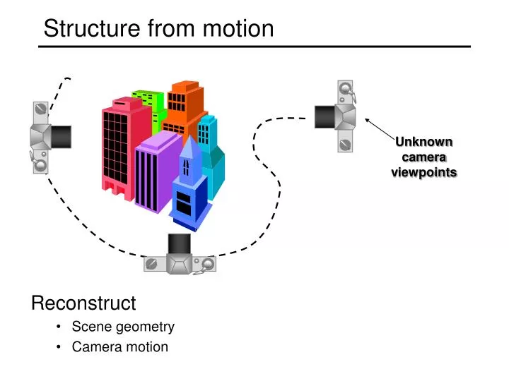
1. Structure from motion • Reconstruct • Scene geometry • Camera motion Unknown camera viewpoints

2. Structure from motion • The SFM Problem • Reconstruct scene geometry and camera motion from two or more images Track 2D Features Estimate 3D Optimize (Bundle Adjust) Fit Surfaces SFM Pipeline

3. Structure from motion • Step 1: Track Features • Detect good features • corners, line segments • Find correspondences between frames • Lucas & Kanade-style motion estimation • window-based correlation

4. Structure Images Motion Structure from motion • Step 2: Estimate Motion and Structure • Simplified projection model, e.g., [Tomasi 92] • 2 or 3 views at a time [Hartley 00]

5. Structure from motion • Step 3: Refine Estimates • “Bundle adjustment” in photogrammetry

6. Structure from motion • Step 4: Recover Surfaces • Image-based triangulation [Morris 00, Baillard 99] • Silhouettes [Fitzgibbon 98] • Stereo [Pollefeys 99] Poor mesh Good mesh Morris and Kanade, 2000

7. Feature tracking • Problem • Find correspondence between n features in f images • Issues • What’s a feature? • What does it mean to “correspond”? • How can correspondence be reliably computed?

8. Feature detection • What’s a good feature?

9. Good features to track • Recall Lucas-Kanade equation: • When is this solvable? • ATA should be invertible • ATA should not be too small due to noise • eigenvalues l1 and l2 of ATA should not be too small • ATA should be well-conditioned • l1/ l2 should not be too large (l1 = larger eigenvalue) • These conditions are satisfied when min(l1, l2) > c

10. Feature correspondence • Correspondence Problem • Given feature patch F in frame H, find best match in frame I Find displacement (u,v) that minimizes SSD error over feature region • Solution • Small displacement: Lukas-Kanade • Large displacement: discrete search over (u,v) • Choose match that minimizes SSD (or normalized correlation)

11. Find displacement (u,v) that minimizes SSD error over feature region • Minimize with respect to Wx and Wy • Affine model is common choice [Shi & Tomasi 94] Feature distortion • Feature may change shape over time • Need a distortion model to really make this work

12. Tracking over many frames • So far we’ve only considered two frames • Basic extension to f frames • Select features in first frame • Given feature in frame i, compute position/deformation in i+1 • Select more features if needed • i = i + 1 • If i < f, go to step 2 • Issues • Discrete search vs. Lucas Kanade? • depends on expected magnitude of motion • discrete search is more flexible • How often to update feature template? • update often enough to compensate for distortion • updating too often causes drift • How big should search window be? • too small: lost features. Too large: slow

13. Incorporating dynamics • Idea • Can get better performance if we know something about the way points move • Most approaches assume constant velocity or constant acceleration • Use above to predict position in next frame, initialize search

14. Modeling uncertainty • Kalman Filtering (http://www.cs.unc.edu/~welch/kalman/ ) • Updates feature state and Gaussian uncertainty model • Get better prediction, confidence estimate • CONDENSATION (http://www.dai.ed.ac.uk/CVonline/LOCAL_COPIES/ISARD1/condensation.html ) • Also known as “particle filtering” • Updates probability distribution over all possible states • Can cope with multiple hypotheses

15. Approach • Predict position at time t: • Measure (perform correlation search or Lukas-Kanade) and compute likelihood • Combine to obtain (unnormalized) state probability Probabilistic Tracking • Treat tracking problem as a Markov process • Estimate p(xt | zt, xt-1) • prob of being in state xt given measurement zt and previous state xt-1 • Combine Markov assumption with Bayes Rule measurement likelihood (likelihood of seeing this measurement) prediction (based on previous frame and motion model)

16. prediction measurement posterior prediction Kalman filtering: assume p(x) is a Gaussian • Key • s = x (position) • o = z (sensor) initial state [Schiele et al. 94], [Weiß et al. 94], [Borenstein 96], [Gutmann et al. 96, 98], [Arras 98] Robot figures courtesy of Dieter Fox

17. Modeling probabilities with samples • Allocate samples according to probability • Higher probability—more samples

18. Measurement posterior CONDENSATION [Isard & Blake] Initialization: unknown position (uniform)

19. CONDENSATION [Isard & Blake] • Prediction: • draw new samples from the PDF • use the motion model to move the samples

20. Measurement posterior CONDENSATION [Isard & Blake]

21. Monte Carlo robot localization • Particle Filters [Fox, Dellaert, Thrun and collaborators]

22. CONDENSATION Contour Tracking • Training a tracker

23. CONDENSATION Contour Tracking • Red: smooth drawing • Green: scribble • Blue: pause

24. Structure from motion • The SFM Problem • Reconstruct scene geometry and camera positions from two or more images • Assume • Pixel correspondence • via tracking • Projection model • classic methods are orthographic • newer methods use perspective • practically any model is possible with bundle adjustment

25. image point projection matrix scene point image offset SFM under orthographic projection • Trick • Choose scene origin to be centroid of 3D points • Choose image origins to be centroid of 2D points • Allows us to drop the camera translation: More generally: weak perspective, para-perspective, affine

26. projection of n features in f images W measurement M motion S shape Key Observation: rank(W) <= 3 Shape by factorization [Tomasi & Kanade, 92] projection of n features in one image:

27. solve for known • Factorization Technique • W is at most rank 3 (assuming no noise) • We can use singular value decomposition to factor W: Shape by factorization [Tomasi & Kanade, 92]

28. Singular value decomposition (SVD) • SVD decomposes any mxn matrix A as • Properties • Σ is a diagonal matrix containing the eigenvalues of ATA • known as “singular values” of A • diagonal entries are sorted from largest to smallest • columns of U are eigenvectors of AAT • columns of V are eigenvectors of ATA • If A is singular (e.g., has rank 3) • only first 3 singular values are nonzero • we can throw away all but first 3 columns of U and V • Choose M’ = U’, S’ = Σ’V’T

29. solve for known • Factorization Technique • W is at most rank 3 (assuming no noise) • We can use singular value decomposition to factor W: • S’ differs from S by a linear transformation A: • Solve for A by enforcing metric constraints on M Shape by factorization [Tomasi & Kanade, 92]

30. Trick (not in original Tomasi/Kanade paper, but in followup work) • Constraints are linear in AAT: • Solve for G first by writing equations for every Pi in M • Then G = AAT by SVD (since U = V) Metric constraints • Orthographic Camera • Rows of P are orthonormal: • Weak Perspective Camera • Rows of P are orthogonal: • Enforcing “Metric” Constraints • Compute A such that rows of M have these properties

31. Factorization with noisy data • Once again: use SVD of W • Set all but the first three singular values to 0 • Yields new matrix W’ • W’ is optimal rank 3 approximation of W • Approach • Estimate W’, then use noise-free factorization of W’ as before • Result minimizes the SSD between positions of image features and projection of the reconstruction

32. Many extensions • Independently Moving Objects • Perspective Projection • Outlier Rejection • Subspace Constraints • SFM Without Correspondence

33. Extending factorization to perspective • Several Recent Approaches • [Christy 96]; [Triggs 96]; [Han 00]; [Mahamud 01] • Initialize with ortho/weak perspective model then iterate • Christy & Horaud • Derive expression for weak perspective as a perspective projection plus a correction term: • Basic procedure: • Run Tomasi-Kanade with weak perspective • Solve for i (different for each row of M) • Add correction term to W, solve again (until convergence)

34. Bundle adjustment • 3D → 2D mapping • a function of intrinsics K, extrinsics R & t • measurement affected by noise • Log likelihood of K,R,t given {(ui,vi)} • Minimized via nonlinear least squares regression • called “Bundle Adjustment” • e.g., Levenberg-Marquardt • described in Press et al., Numerical Recipes

35. Match Move • Film industry is a heavy consumer • composite live footage with 3D graphics • known as “match move” • Commercial products • 2D3 • http://www.2d3.com/ • RealVis • http://www.realviz.com/ • Show video

36. Closing the loop • Problem • requires good tracked features as input • Can we use SFM to help track points? • basic idea: recall form of Lucas-Kanade equation: • with n points in f frames, we can stack into a big matrix • Matrix on RHS has rank <= 3 !! • use SVD to compute a rank 3 approximation • has effect of filtering optical flow values to be consistent • [Irani 99]

37. From [Irani 99]

38. References • C. Baillard & A. Zisserman, “Automatic Reconstruction of Planar Models from Multiple Views”, Proc. Computer Vision and Pattern Recognition Conf. (CVPR 99) 1999, pp. 559-565. • S. Christy & R. Horaud, “Euclidean shape and motion from multiple perspective views by affine iterations”, IEEE Transactions on Pattern Analysis and Machine Intelligence, 18(10):1098-1104, November 1996 (ftp://ftp.inrialpes.fr/pub/movi/publications/rec-affiter-long.ps.gz ) • A.W. Fitzgibbon, G. Cross, & A. Zisserman, “Automatic 3D Model Construction for Turn-Table Sequences”, SMILE Workshop, 1998. • M. Han & T. Kanade, “Creating 3D Models with Uncalibrated Cameras”, Proc. IEEE Computer Society Workshop on the Application of Computer Vision (WACV2000), 2000. • R. Hartley & A. Zisserman, “Multiple View Geometry”, Cambridge Univ. Press, 2000. • R. Hartley, “Euclidean Reconstruction from Uncalibrated Views”, In Applications of Invariance in Computer Vision, Springer-Verlag, 1994, pp. 237-256. • M. Isard and A. Blake, “CONDENSATION -- conditional density propagation for visual tracking”, International Journal Computer Vision, 29, 1, 5--28, 1998. (ftp://ftp.robots.ox.ac.uk/pub/ox.papers/VisualDynamics/ijcv98.ps.gz ) • S. Mahamud, M. Hebert, Y. Omori and J. Ponce, “Provably-Convergent Iterative Methods for Projective Structure from Motion”,Proc. Conf. on Computer Vision and Pattern Recognition, (CVPR 01), 2001. (http://www.cs.cmu.edu/~mahamud/cvpr-2001b.pdf ) • D. Morris & T. Kanade, “Image-Consistent Surface Triangulation”, Proc. Computer Vision and Pattern Recognition Conf. (CVPR 00), pp. 332-338. • M. Pollefeys, R. Koch & L. Van Gool, “Self-Calibration and Metric Reconstruction in spite of Varying and Unknown Internal Camera Parameters”, Int. J. of Computer Vision, 32(1), 1999, pp. 7-25. • J. Shi and C. Tomasi, “Good Features to Track”, IEEE Conf. on Computer Vision and Pattern Recognition (CVPR 94), 1994, pp. 593-600 (http://www.cs.washington.edu/education/courses/cse590ss/01wi/notes/good-features.pdf ) • C. Tomasi & T. Kanade, ”Shape and Motion from Image Streams Under Orthography: A Factorization Method", Int. Journal of Computer Vision, 9(2), 1992, pp. 137-154. • B. Triggs, “Factorization methods for projective structure and motion”, Proc. Computer Vision and Pattern Recognition Conf. (CVPR 96), 1996, pages 845--51. • M. Irani, “Multi-Frame Optical Flow Estimation Using Subspace Constraints”, IEEE International Conference on Computer Vision (ICCV), 1999 (http://www.wisdom.weizmann.ac.il/~irani/abstracts/flow_iccv99.html )