
Mastering Morphological Image Processing Techniques
E N D
Presentation Transcript
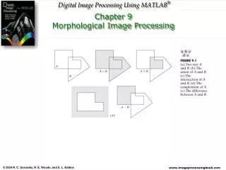
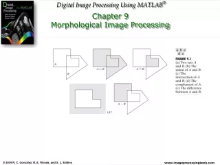
Morphological Image Processing • Mathematical morphology is a tool for extracting image components that are useful in the representation and description of region shape, such as boundaries, skeletons, and the convex hull. • We are also interested in morphological techniques for pre- or post processing, such as morphological filtering, thinning, and pruning. • We begin the discussion of morphology by studying two operations: erosion and dilation.
Erosion and Dilation • These operations are fundamental to morphological processing. • In fact, many of the morphological algorithms discussed in this chapter are based on these two primitive operations.
Erosion • A ⊖ B: erosion of A by B where B is assumed to be the structuring element. • It is typically applied to binary images, but there are versions that work on gray scale images. • The basic effect of the operator on a binary image is to erode away the boundaries of regions of foreground pixels (i.e. white pixels, typically). Thus areas of foreground pixels shrink in size, and holes within those areas become larger.
Erosion • Suppose that we wish to remove the lines connecting the center region to the border pads in fig. 9.5(a). Eroding the image with square structuring element of size 11 x 11 whose components are all 1s removed most of the lines as fig. 9.5(b). Shows. The reason the two vertical lines in the center were thinned but not removed completely because their width is greater than 11. changing the SE to 15 x 15 and eroding the original image again removed all the connecting lines. Then a SE of 45 x 45 is used which eliminated all other lines. • Erosion shrinks or thins objects in a binary image • All image details smaller that the structuring element are filtered from the image.
Dilation • A ⊕ B: the dilation of A by B where B is assumed to be the structuring element. • Unlike erosion which is a shrinking or thinning operation, dilation “grows” or “thickens” objects in a binary image. • The specific manner or the extent of this thickness is controlled by the shape of the structuring element used. • One of the simplest applications of dilation is for bridging gaps.
Opening and Closing • Opening generally smooths the contour of an object • Opening denoted as: A ∘ B = (A ⊖ B) ⊕ B . • Breaks narrow isthmuses, and eliminates thin protrusions. • Closing also tends to smooth sections of contours but, as opposed to opening, it generally fuses narrow breaks and long thin gulfs, eliminate holes, and fills gaps in the contour. • Closing denoted as: A ∙ B=(A ⊕ B) ⊖ B
Fig.9.10 illustrates the openning and closing operations • Fig. 9.10(a) shows a set A, and Fig. 9.10(b) shows various positions of a disk structuring element during the erosion process. • When completed, this process resulted in disjoint figure 9.10( c ). Note the elimination of the bridge between the two main sections. • Fig.9.10(d) shows the process of dilating the eroded set • Fig.9.10(e) shows the final result of opening. Note that outward pointing corners were rounded, where as inward pointing corners were not affected. • Similarly, Figs. 9.10(f) through (i) show the results of closing A with the same structuring element. We note that the inward pointing corners were rounded, where as the outward pointing corners remained unchanged. The left most intrusion on the boundary of A was reduced in sizebecause the disk did’nt fit in there.
Fig. 9.11 Discussion • Morphological operations can be used as spatial filters. • The binary image in Fig.9.11(a) shows a section of fingerprint corrupted by noise • The objective here is to eliminate the noise using a morphological filter consisting of opening followed by closing. • Fig. 9.11(b) shows the structuring element used. • Fig.9.11( c ) is the result of eroding A with the structuring element. The background noise was completely eleminated in the erosion stage of opening in this case all noise components are smaller than the structuring element. • In Fig.9.11(d) shows the dilation operation on Fig. (c ) the noise components in fingerprint were reduced in size or deleted completely. • In Fig(e) most of line breaks were restored but the ridges were thickened a condition that can be remedied by erosion the result shown in Fig.(f).
Some Basic Morphological Algorithms • We are now ready to consider some practical uses of morphology. • When dealing with binary images, one of the principal applications of morphology is in extracting image components that are useful in the representation and description of shape. • In particular, we consider morphological algorithms for extracting boundaries, connecting components, the convex hull, and the skeleton of a region. • We also develop several methods for region filling, thinning, thickening, and pruning that are used frequently in conjunction with these algorithms as pre- or post- processing steps.
Some Basic Morphological Algorithms • Boundary Extraction • Hole Filling • Extraction of connected Components • Convex Hull
Boundary Extraction • The boundary of a set A, denoted by β(A), can be obtained by first eroding A by B and then performing the set difference between A and its erosion. That is: β(A) = A – (A ⊖ B)………….. Eq.(9.5-1) Where B is a suitable structuring element.
Boundary Extraction • Fig. 9.13 illustrates the mechanics of boundary extraction. It shows a simple binary object, a structuring element B, and the result of using Eq.(9.5-1).
Boundary Extraction • Fig.9.14 illustrates the use of Eq.(9.5-1). • With a 3 x 3 structuring element of 1s. As for all binary images in this chapter, binary 1s are shown in white and 0s in black. • so the elements of the structuring element, which are 1s, also are treated as white. • Because of the size of the structuring element used, the boundary in Fig.9.14(b) is one pixel thick.
Hole Filling • A hole may be defined as a background region surrounded by a connected border of foreground pixels. • In this section an algorithm is developed based on set dilation, complementation, and intersection for filling holes in an image. • Let A denote a set whose elements are 8-connected boundaries, such boundary enclosing a background region (i.e., a hole). Given a point in each hole, the objective is to fill the holes with 1s. • We begin by forming an array X 0, of 0s (the same size as the array containing A), except at the locations in X 0 corresponding to the given point in each hole, which we set to 1, then the following procedure fills all the holes with 1s: • X k = (Xk-1 ⊕ B) ∩ Ac ) k = 1,2,3,… Eq(9.5-2)
Hole Filling • Where B is the symmetric structuring element in Fig.9.15(c). • The algorithm terminates at iteration step K if X k = X k-1. • the set X k then contains all the filled holes. • The set union of X k and A contains all the filled holes and their boundaries. • The dilation of E1.(9.5-2) would fill the entire area if left unchecked. However, the intersection at each step with Ac limits the result to inside the region of interest. • This is the first example of how a morphological process can be conditioned to meet a desired property. • In the current application, it is called conditional dilation. • The rest of Fig.9.15 illustrates further the mechanics of Eq.(9.5-2). Although this example only has one hole, the concept clearly applies to any finite number of holes.
Extraction of connected components • Extraction of connected components from a binary image central to many automated image analysis applications. • The objective is to start with X 0 and find all the connected components. • The following algorithm accomplishes this objective: • X k = (Xk-1 ⊕ B) ∩ A ) k = 1,2,3,… Eq(9.5-3) • Where B is a suitable structuring element. • Note that similarity in Eqa(9.5-2) and (9.5-3), the only difference being the use of A as opposed to Ac . This is not surprising, because here we are looking for foreground points, while the objective in section 9.5.2 was to find the background point.
Extraction of connected components • Fig.9.17 illustrates the mechanics of Eq.(9.5-3). With convergence being achieved for k = 6. • Note that the shape of the structuring element used is based on 8-connectivity between pixels. • If we had used the previous SE with 4-connectivity not all the pixels will be detected especially the leftmost ones.
The Hit-or-Miss Transformations • The morphological hit-or-miss transform is a basic tool for shape detection. A ⊛ B = (A ⊖ B1) – (A ⊕ B2) • The reason of using two structuring elements B1,B2.while B1is associated with objects and B2associated with the background. • The hit-and-miss transform is a general binary morphological operation that can be used to look for particular patterns of foreground and background pixels in an image. • It is actually the basic operation of binary morphology since almost all the other binary morphological operators can be derived from it. • As with other binary morphological operators it takes as input a binary image and a structuring, and produces another binary image as output.
Thinning • The thinning of a set A by a structuring element B, denoted by: A ⊗ B = A – (A ⊛ B) = A ∩ (A ⊛ B)c • The thinning algorithm is based on a sequence of structuring elements: • {B} = {B1,B2,B3,…Bn} • Where Bi is a rotated version of Bi-1 . Using this concept, we now define thinning by a sequence of structuring elements as: A ⊗ {B} = ((…((A ⊗ B1) ⊗ B2 )…) ⊗ Bn ) • The process is to thin A by one pass with B1 , then thin the result with one pass of B2, and so on, until A is thinned with one pass of Bn . The entire process is repeated until no further changes occur.
Thinning • Figure 9.21(a) shows a set of structuring elements commonly used for thinning. • Fig. 9.21(b) shows a set A to be thinned by using the procedure just discussed. • Fig.9.21(c) shows the result of thinning after one pass of A with B1 . • Figs.9.21(d) through (k) show the results of passes with the other structuring elements.
Thickening • Thickening is the morphological dual of thinning and is defined by the expression: A ⊙ B = A ⋃ (A ⊛ B) • Where B is a structuring element suitable for thickening. As in thinning, thickening can be defined as a sequential operation: A ⊙{B} = ((…((A ⊙B1) ⊙B2 )…) ⊙Bn) • The structuring elements used for thickening have the same form as those shown in Fig.9.21(a), but with all 1s and 0s interchanged.
Thickening • A separate algorithm for thickening is seldom used in practice. • Instead, the usual procedure is to thin the background of the set in question and then complement the result. • In other words, to thicken a set A, we form C = Ac , thin C, and then form Cc. • Figure. 9.22 illustrates this procedure.
Skeleton • Skeletonization is a process for reducing foreground regions in a binary image to a skeletal remnant that largely preserves the extent and connectivity of the original region while throwing away most of the original foreground pixels. • Under this definition it is clear that thinning produces a sort of skeleton.
Pruning • Pruning methods are an essential complement to thinning and skeletonizing algorithms because these procedures tend to leave parasitic components that need to be “cleaned up” by post processing. • We begin the discussion with a pruning problem and then develop a morphological solution based on the material introduced in the preceding sections. • Thus we take this opportunity to illustrate how to go about solving a problem by combining several of the techniques discussed up to this point.
Pruning • A common approach in the automated recognition of hand-printed characters is to analyze the shape of the skeleton of each character. • These skeletons often are characterized by “spurs” (parasitic components). • We develop a morphological technique for handling this problem. • Fig.9.25(a) shows the skeleton of a hand-printed “a”. The parasitic component is in the left most part of the character where we are intrested in removing.
Pruning • The solution is based on suppressing a parasitic branch by successively eliminating its end points. • Thinning of an input set A with a sequence of structuring elements designed to detect only end points achieves the desired result.