Download
1 / 83
830 likes | 860 Views
Learn about heuristic functions derived from relaxed models to simplify complex problems, with examples such as road navigation and the Tile Puzzle problem, along with the STRIPS Problem formulation and methods like pattern databases. Understand admissibility and consistency in heuristics, and explore cost functions in best-first search algorithms like A*.

E N D
Chapter 6 Origin of Heuristic Functions
Heuristic from Relaxed Models • A heuristic function returns the exact cost of reaching a goal in a simplified or relaxed version of the original problem. • This means that we remove some of the constraints of the problem. • Removing constraints = adding edges
Example: Road navigation • A good heuristic – the straight line. • We remove the constraint that we have to move along the roads • We are allowed to move in a straight line between two points. • We get a relaxation of the original problem. • In fact, we added edges of the complete graph
Example 2: - TSP problem • We can describe the problem as a graph with 3 constraints: 1) Our tour covers all the cities. 2) Every node has a degree two • an edge entering the node and • an edge leaving the node. 3) The graph is connected. • If we remove constraint 2 : We get a spanning graph and the optimal solution to this problem is a MST (Minimum Spanning Tree). • If we remove constraint 3: Now the graph isn’t connected and the optimal solution to this problem is the solution to the assignment problem.
Example 3- Tile Puzzle problem • One of the constraints in this problem is that a tile can only slide into the position occupied by a blank. • If we remove this constraint we allow any tile to be moved horizontally or vertically position. • This is the Manhattan distance to its goal location.
The STRIPS Problem formulation • We would like to derive such heuristics automatically. • In order to do that we need a formal description language that is richer than the problem space graph. • One such language is calledSTRIPS. • In this language we have predicates and operators. • Let’s see a STRIPS representation of the Eight Puzzle Problem
STRIPS - Eight Puzzle Example • On(x,y) = tile x is in location y. • Clear(z) = location z is clear. • Adj(y,z) = location y is adjacent to location z. • Move(x,y,z) = move tile x from location y to location z. In the language we have: • A precondition list - for example to execute move(x,y,z) we must have: On(x,y) Clear(z) Adj(y,z) • An add list - predicates that weren’t true before the operator and now after the operator was executed are true. • A delete list - a subset of the preconditions, that now after the • operator was executed aren’t true anymore.
STRIPS - Eight Puzzle Example • Now in order to construct a simplified or relaxed problem we only have to remove some of the preconditions. • For example - by removing Clear(z) we allow tiles to move to adjacent locations. • In general, the hard part is to identify which relaxed problems have the property that their exact solution can be efficiently computed.
Admissibility and Consistency • The heuristics that are derived by this method are both admissible and consistent. • Note : The cost of the simplified graph should be as close as possible to the original graph. • Admissibility means that the simplified graph has an equal or lower cost than the lowest - cost path in the original graph. • Consistency means that a heuristic h is consistent for every neighbor n’ of n, • when h(n) is the actual optimal cost of reaching a goal in the graph of the relaxed problem. h(n) c(n,n’)+h(n’)
Method 2: pattern data base • A different method for abstracting and relaxing to problem to get a simplified problem. • Invented in 1996 by Culberson & Schaeffer
optimal path search algorithms • For small graphs: provided explicitly, algorithm such as Dijkstra’s shortest path, Bellman-Ford or Floyd-Warshal. Complexity O(n^2). • For very large graphs , which are implicitly defined, the A* algorithm which is a best-first search algorithm.
Best-first search schema • sorts all generated nodes in an OPEN-LIST and chooses the node with the best cost value for expansion. • generate(x): insert x into OPEN_LIST. • expand(x): delete x from OPEN_LIST and generate its children. • BFS depends on its cost (heuristic) function. Different functions cause BFS to expand different nodes.. 20 25 30 30 35 35 35 40 Open-List
Best-first search: Cost functions • g(x):Real distance from the initial state to x • h(x): The estimated remained distance from x to the goal state. • Examples:Air distance Manhattan Dinstance Different cost combinations of g and h • f(x)=level(x) Breadth-First Search. • f(x)=g(x) Dijkstra’s algorithms. • f(x)=h’(x) Pure Heuristic Search (PHS). • f(x)=g(x)+h’(x) The A* algorithm (1968).
A* (and IDA*) • A* is a best-first search algorithm that uses f(n)=g(n)+h(n)as its cost function. • f(x) in A* is an estimation of the shortest path to the goal via x. • A* is admissible, complete and optimally effective. [Pearl 84] • Result: any other optimal search algorithm will expand at least all the nodes expanded by A* Breadth First Search A*
1 2 3 1 2 3 4 4 5 6 7 5 6 7 8 9 8 9 10 11 10 11 12 13 14 12 13 14 15 15 16 17 18 19 20 21 22 23 24 Domains 15 puzzle • 10^13 states • First solved by [Korf 85] with IDA* and Manhattan distance • Takes 53 seconds 24 puzzle • 10^24 states • First solved by [Korf 96] • Takes two days
Domains • Rubik’s cube • 10^19 states • First solved by [Korf 97] • Takes 2 days to solve
1 2 3 4 5 N (n,k) Pancake Puzzle • An array of N tokens (Pancakes) • Operators: Any first k consecutive tokens can be reversed. • The 17 version has 10^13 states • The 20 version has 10^18 states
(n,k) Top Spin Puzzle • n tokens arranged in a ring • States: any possible permutation of the tokens • Operators: Any k consecutive tokens can be reversed • The (17,4) version has 10^13 states • The (20,4) version has 10^18 states
4-peg Towers of Hanoi (TOH4) • Harder than the known 3-peg Towers of Hanoi • There is a conjecture about the length of optimal path but it was not proven. • Size 4^k
How to improve search? • Enhanced algorithms: • Perimeter-search [Delinberg and Nilson 95] • RBFS [Korf 93] • Frontier-search [Korf and Zang 2003] • Breadth-first heuristic search [Zhou and Hansen 04] They all try to better explore the search tree. • Better heuristics:more parts of the search tree will be pruned.
Better heuristics • In the 3rd Millennium we have very large memories. We can build large tables. • For enhanced algorithms: large open-lists or transposition tables. They store nodes explicitly. • A more intelligent way is to store general knowledge. We can do this with heuristics
Subproblems-Abstractions • Many problems can be abstracted into subproblems that must be also solved. • A solution to the subproblem is a lower bound on the entire problem. • Example: Rubik’s cube [Korf 97] • Problem: 3x3x3 Rubik’s cube Subproblem: 2x2x2 Corner cubies.
Pattern Databases heuristics • A pattern database (PDB) is a lookup table that stores solutions to all configurations of the sub-problem (patterns) • This PDB is used as a heuristic during the search 88 Million states 10^19 States Search space Mapping/Projection Pattern space
Non-additive pattern databases • Fringe pattern database[Culberson & Schaeffer 1996]. • Has only 259 Million states. • Improvement of a factor of 100 over Manhattan Distance
Example - 15 puzzle 1 1 4 5 10 4 5 8 11 9 12 2 13 15 8 9 10 11 3 6 714 12 13 14 15 • How many moves do we need to move tiles 2,3,6,7 from locations 8,12,13,14 to their goal locations • The solution to this is located in PDB[8][12][13][14]=18
Example - 15 puzzle 2 3 6 7 • How many moves do we need to move tiles 2,3,6,7 from locations 8,12,13,14 to their goal locations • The solution to this is located in PDB[8][12][13][14]=18
7-8 Disjoint Additive PDBs (DADB) • If you have many PDBS, take their maximum • Values of disjointdatabases can be added and are still admissible [Korf & Felner: AIJ-02, Felner, Korf & Hanan: JAIR-04] • Additivity can be applied if the cost of a subproblem is composed from costs of objects from corresponding pattern only
DADB:Tile puzzles 5-5-5 6-6-3 7-8 6-6-6-6 [Korf, AAAI 2005]
Heuristics for the TOH • Infinite peg heuristic (INP): Each disk moves to its own temporary peg. • Additive pattern databases [Felner, Korf & Hanan, JAIR-04]
Additive PDBS for TOH4 • Partition the disks into disjoint sets • Store the cost of the complete pattern space of each set in a pattern database. • Add values from these PDBs for the heuristic value. • The n-disk problem contains 4^n states • The largest database that we stored was of 14 disks which needed 4^14=256MB. 6 10
TOH4: results • The difference between static and dynamic is covered in [Felner, Korf & Hanan: JAIR-04]
Best Usage of Memory • Given 1 giga byte of memory, how do we best use it with pattern databases? • [Holte, Newton, Felner, Meshulam and Furcy, ICAPS-2004] showedthat it is better to use many small databases and take their maximum instead of one large database. • We will present a different (orthogonal) method [Felner, Mushlam & Holte: AAAI-04].
Compressing pattern database Felner et al AAAI-04]] • Traditionally, each configuration of the pattern had a unique entry in the PDB. • Our main claim Nearby entries in PDBs are highly correlated !! • We propose to compress nearby entries by storing their minimum in one entry. • We show that most of the knowledge is preserved • Consequences: Memory is saved, larger patterns can be used speedup in search is obtained.
Cliques in the pattern space • The values in a PDB for a clique are d or d+1 • In permutation puzzles cliques exist when only one object moves to another location. d G d+1 d • Usually they have nearby entries in the PDB • A[4][4][4][4][4] A clique in TOH4
Compressing cliques • Assume a clique of size K with values d or d+1 • Store only one entry (instead of K) for the clique with the minimum d.Lose at most 1. • A[4][4][4][4][4] A[4][4][4][4][1] • Instead of 4^p we need only 4^(p-1) entries. • This can be generalized to a set of nodes with diameter D. (for cliques D=1) • A[4][4][4][4][4] A[4][4][4][1][1] • In general: compressing by k disks reduces memory requirements from 4^pto4^(p-k)
TOH4 results: 16 disks (14+2) • Memory was reduced by a factor of 1000!!! at a cost of only a factor of 2 in the search effort.
Memory was reduced by a factor of 1000!!! At a cost of only a factor of 2 in the search effort. Lossless compressing is noe efficient in this domain. TOH4: larger versions • For the 17 disks problem a speed up of 3 orders of magnitude is obtained!!! • The 18 disks problem can be solved in 5 minutes!!
Tile Puzzles Goal State Clique • Storing PDBs for the tile puzzle • (Simple mapping) A multi dimensional array A[16][16][16][16][16] size=1.04Mb • (Packed mapping) One dimensional array A[16*15*14*13*12 ] size = 0.52Mb. • Time versus memory tradeoff !!
15 puzzle results • A clique in the tile puzzle is of size 2. • We compressed the last index by two A[16][16][16][16][8]
Symmetries in PDBs • Symmetric lookups were already performed by the first PDB paper of [Culberson & Schaeffer 96] • examples • Tile puzzles: reflect the tiles about the main diagonal. • Rubik’s cube: rotate the cube • We can take the maximum among the different lookups • These are all geometricalsymmetries • We suggest a new type of symmetry!! 7 8 7 8
Regular and dual representation • Regular representation of a problem: • Variables – objects (tiles, cubies etc,) • Values – locations • Dualrepresentation: • Variables – locations • Values – objects
Regular vs. Dual lookups in PDBs • Regular question: Where are tiles {2,3,6,7} and how many moves are needed to gather them to their goal locations? • Dual question: Who are the tiles in locations {2,3,6,7} and how many moves are needed to distribute them to their goal locations?
Regular and dual lookups • Regular lookup: PDB[8,12,13,14] • Dual lookup: PDB[9,5,12,15]
Regular and dual in TopSpin • Regular lookup for C : PDB[1,2,3,7,6] • Dual lookup for C: PDB[1,2,3,8,9]
Dual lookups • Dual lookups are possible when there is a symmetry between locations and objects: • Each object is in only one location and each location occupies only one object. • Good examples: TopSpin, Rubik’s cube • Bad example: Towers of Hanoi • Problematic example: Tile Puzzles
Inconsistency of Dual lookups • Consistency of heuristics: • |h(a)-h(b)| <= c(a,b) Example:Top-Spin c(b,c)=1 • Both lookups for B PDB[1,2,3,4,5]=0 • Regular lookup for C PDB[1,2,3,7,6]=1 • Dual lookup for C PDB[1,2,3,8,9]=2
Traditional Pathmax • children inherit f-value from their parents if it makes them larger g=1 h=4 f=5 Inconsistency g=2 h=2 f=4 g=2 h=3 f=5 Pathmax
Bidirectional pathmax (BPMX) h-values h-values 2 4 BPMX 5 1 5 3 • Bidirectional pathmax: h-values are propagated in both directions decreasing by 1 in each edge. • If the IDA* threshold is 2 then with BPMX the right child will not even be generated!!
Results: (17,4) TopSpin puzzle • Nodes improvement (17r+17d) : 1451 • Time improvement (4r+4d) : 72 • We also solved the (20,4) TopSpin version.