8. Association between Categorical Variables

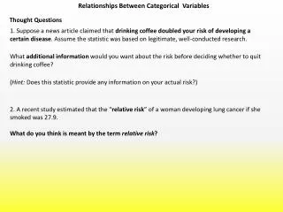
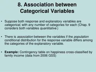
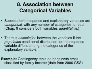
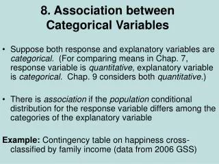
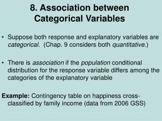
1. 8. Association between Categorical Variables • Suppose both response and explanatory variables are categorical. (Chap. 9 considers both quantitative.) • There is association if the population conditional distribution for the response variable differs among the categories of the explanatory variable Example: Contingency table on happiness cross-classified by family income (data from 2006 GSS)

2. Happiness Income Very Pretty Not too Total --------------------------------------------- Above 272 (44%) 294 (48%) 49 (8%) 615 Average 454 (32%) 835 (59%) 131 (9%) 1420 Below 185 (20%) 527 (57%) 208 (23%) 920 ---------------------------------------------- Response: Happiness, Explanatory: Income The sample conditional distributions on happiness vary by income level, but can we conclude that this is also true in the population?

3. Guidelines for Contingency Tables • Show sample conditional distributions: percentages for the response variable within the categories of the explanatory variable. Find by dividing the cell counts by the explanatory category total and multiplying by 100. (Percents on response categories will add to 100) • Clearly define variables and categories. • If display percentages but not the cell counts, include explanatory total sample sizes, so reader can (if desired) recover all the cell count data. (I use rows for explanatory var., columns for response var.)

4. Independence & Dependence • Statistical independence (no association): Population conditional distributions on one variable the same for all categories of the other variable • Statistical dependence (association): Conditional distributions are not all identical Example of statistical independence: Happiness Income Very Pretty Not too ----------------------------------------- Above 32% 55% 13% Average 32% 55% 13% Below 32% 55% 13%

5. Chi-Squared Test of Independence (Karl Pearson, 1900) • Tests H0: The variables are statistically independent • Ha: The variables are statistically dependent • Intuition behind test statistic: Summarize differences between observed cell counts and expected cell counts (what is expected if H0 true) • Notation: fo = observed frequency (cell count) fe = expected frequency r = number of rows in table, c = number of columns

6. Expected frequencies (fe): • Have identical conditional distributions. Those distributions are same as the column (response) marginal distribution of the data. • Have same marginal distributions (row and column totals) as observed frequencies • Computed by fe = (row total)(column total)/n

7. Happiness Income Very Pretty Not too Total -------------------------------------------------- Above 272 (189.6) 294 (344.6) 49 (80.8) 615 Average 454 (437.8) 835 (795.8) 131 (186.5) 1420 Below 185 (283.6) 527 (515.6) 208 (120.8) 920 -------------------------------------------------- Total 911 1656 388 2955 e.g., first cell has fe= 615(911)/2955 = 189.6. fe values are in parentheses in this table

8. Chi-Squared Test Statistic • Summarize closeness of {fo} and {fe} by with sum is taken over all cells in the table. • When H0 is true, sampling distribution of this statistic is approximately (for large n) the chi-squared probability distribution.

9. Properties of chi-squared distribution • On positive part of line only • Skewed to right (more bell-shaped as df increases) • Mean and standard deviation depend on size of table through df = (r – 1)(c – 1) = mean of distribution, where r = number of rows, c = number of columns • Larger values incompatible with H0,so P-value = right-tail probability above observed test statistic value.

10. Example: Happiness and family income df = (3 – 1)(3 – 1) = 4. P-value = 0.000 (rounded, often reported as P < 0.001). Chi-squared percentile values for various right-tail probabilities are in table on text p. 594. There is very strong evidence against H0: independence (namely, if H0 were true, prob. would be < 0.001 of getting this large a test statistic or even larger). For significance level  = 0.05 (or  = 0.01 or  = 0.001), we reject H0 and conclude an association exists between happiness and income.

11. Software output (SPSS)

12. Comments about chi-squared test • Using chi-squared dist. to approx the actual sampling dist of the test statistic works well for “large” random samples. (Cochran (1954) showed it works ok in practice if all or nearly all fe≥ 5) • For smaller samples, Fisher’s exact test applies (we skip) • Most software also reports “likelihood-ratio chi squared,” an alternative chi-squared test statistic. • Chi-squared test treats variables as nominal scale (re-order categories, get same result). For ordinal variables, more powerful tests are available (such as in Sections 8.5 and 8.6 of text), which we skip. We’ll use regression methods in Ch. 9. (Coming soon: Analysis of Ordinal Categorical Data, 2nd ed.)

13. df = (r – 1)(c - 1) means that for given marginal counts, a block of size (r – 1)(c – 1) cell counts determines the other counts. (Ronald Fisher 1922; Pearson, in 1900, said df = rc - 1) • If z is a statistic that has a standard normal dist., then z2 has a chi-squared distribution with df = 1. • For df = d, chi-squared stat’s are equivalent to squaring and summing d independent z stat’s.

14. For 2-by-2 tables, chi-squared test of independence (which has df = 1) is equivalent to testing H0: 1 = 2 for comparing two population proportions, 1 and 2 . Response variable Group Outcome 1 Outcome 2 1 1 1 - 1 2 2 1 -2 H0: 1 = 2 equivalent to H0: response variable independent of group variable Then, chi-squared statistic is square of z test statistic, z = (difference between sample proportions)/(se0).

15. Example (from Chap. 7): College Alcohol Study conducted by Harvard School of Public Health “Have you engaged in unplanned sexual activities because of drinking alcohol?” 1993: 19.2% yes of n = 12,708 2001: 21.3% yes of n = 8783 Results refer to 2-by-2 contingency table: Response Year Yes No Total 1993 2440 10,268 12,708 2001 1871 6912 8783 Pearson 2= 14.3, df = 1, P-value = 0.000 (actually 0.00016) Corresponding z test statistic = 3.78, has (3.78)2 = 14.3.

16. Residuals: Detecting Patterns of Association • Large chi-squared implies strong evidence of association but does not tell us about nature of association. We can investigate this by finding the residual in each cell of the contingency table. • Residual = fo-fe is positive (negative) when there are more (fewer) observations in cell than null hypothesis of independence predicts. • Standardized residualz = (fo-fe)/se, where se denotes se of fo-fe.. This measures number of standard errors that (fo-fe) falls from value of 0 expected when H0 true.

17. The se value is found using So, the standardized residual equals Example: For cell with fo = 272, fe = 189.6, row prop. = 615/2955 = 0.208, column prop. = 911/2955 = 0.308, and standardized residual Number of people with above average income and very happy is 8 standard errors higher than we would expect if happiness were independent of income.

18. SPSS Output

19. Likewise, we see more people in the (below average, not too happy) cell than expected, and fewer in (below average, very happy) and (above average, not too happy) cells than expected. • In cells having |standardized residual| > about 3, departure from independence is noteworthy (probably not just due to “chance”). • Standardized residuals can be found using some software (called adjusted residuals in SPSS). • For 2-by-2 tables, each standardized residual is the same in absolute value (and is a z statistic for comparing two population proportions) and satisfies z2 = 2 (df = 1, and there is only 1 nonredundant residual)

20. Example: “Have you engaged in unplanned sexual activities because of drinking alcohol?” We found Pearson chi-squared = 14.3, P-value < 0.0002 Standardized residuals are: Year Yes No 1993 2440 (-3.78) 10,268 (3.78) • 1871 (3.78) 6912 (-3.78) for which (3.78)2 = 14.3

21. A couple more happiness analyses • Happiness and religiosity(attend religious services 1 = at most several times a year, 2 = once a month to nearly every week, 3 = every week to several times a week), 2006 GSS 2 = 73.5, df = 4, P-value = 0.000. Happiness Religiosity Not too Pretty Very 1 189 (3.9) 908 (4.4) 382 (-7.3) 2 53 (-0.8) 311 (-0.2) 180 (0.8) 3 46 (-3.8) 335 (-4.8) 294 (7.6)

22. Similar results for variables positively correlated with religiosity, such as political conservatism • Happiness and number of sex partners in previous year (2006 GSS) Happiness Sex partners Not too Pretty Very 0 112 (5.9) 329 (-0.9) 154 (-3.2) 1 118 (-7.8) 832 (-1.0) 535 (6.5) At least 2 57 (3.7) 198 (2.5) 57 (-5.3)

23. Measures of Association • Chi-squared test answers “Is there an association?” • Standardized residuals answer “How do data differ from what independence predicts?” • We answer “How strong is the association?” using a measure of the strength of association, such as the difference of proportions

24. Example: Opinion about George W. Bush performance as President (9/08 Gallup poll) Opinion (n about 1000) Political partyApprove Disapprove Democrats 3% 97% Republicans 64% 36% Gender Approve Disapprove Women 24% 76% Men 27% 73% The difference of proportions 0.64 – 0.03 = 0.61 indicates a much stronger association between political party and opinion than the difference 0.27 – 0.24 = 0.03 indicates for gender and opinion.

25. The greater the value of the stronger the association • For r-by-c tables, other summary measures exist (pp. 238-243), but we usually learn more by using the difference of proportions to compare particular levels of one variable in terms of the proportion in a particular category of the other variable. Example: Happiness Income Very Pretty Not too Above 272 (44%) 294 (48%) 49 (8%) Average 454 (32%) 835 (59%) 131 (9%) Below 185 (20%) 527 (57%) 208 (23%) Comparing those of above average income with those of below average income, the difference in the estimated proportion who are “very happy” is 0.44 – 0.20 = 0.24.

26. Comparisons using ratios • Recall the ratio of proportions can also be useful (“relative risk”) Example: Comparing proportions who report being very happy, for those of above average income to those of below average income, 0.44/0.20 = 2.2 An alternative measure for comparing proportions, commonly used for logistic regression model for categorical response variables, is the odds ratio.

27. The “odds” • For two outcomes (“success”, “failure”) for a group, Odds = P(success)/P(failure) = P(success)/[1 - P(success)] e.g., if P(success) = 0.80, P(failure) = 0.20, the odds = 0.80/0.20 = 4.0 if P(success) = 0.20, P(failure) = 0.80, the odds = 0.20/0.80 = ¼ = 0.25 Probability of success obtained from odds by Probability = odds/(odds + 1) e.g., odds = 4.0 has probability = 4/(4+1) = 4/5 = 0.80

28. The odds ratio • For 2 groups summarized in a 2x2 contingency table, odds ratio = (odds in row 1)/(odds in row 2) Example: Survey of senior high school students Alcohol use Cigarette use Yes No Yes 1449 46 No 500 281 2 = 451.4, df = 1 (P-value = 0.00000…..) Standardized residuals all equal +21.2 or – 21.2.

29. For those who have smoked, the odds of having used alcohol are 1449/46 = 31.50. • For those who have not smoked, the odds of having used alcohol are 500/281 = 1.78 • The odds ratio = 31.5/1.78 = 17.7 The estimated odds that smokers have used alcohol are 17.7 times the estimated odds that non-smokers have used alcohol.

30. Properties of the odds ratio • Takes same value regardless of choice of response variable. Example: The estimated odds that alcohol users have smoked are (1449/500)/(46/281) = 2.90/0.163 = 17.7 times estimated odds that non-alcohol users smoked. • Takes nonnegative values, with odds ratio = 1.0 corresponding to “no effect” and odds ratio values farther from 1.0 representing stronger associations.

31. Can be computed as a cross-product ratio (Yule 1900). Example: Alcohol use Cigarette use Yes No Total Yes 1449 46 1495 No 500 281 781 odds ratio = (1449)(281)/(46)(500) = 17.7 • Note the odds ratio is a ratio of odds, not a ratio of proportions like the relative risk. E.g., for alcohol use as response variable, relative risk = (1449/1495)/(500/781) = 0.97/0.64 = 1.5 For those who’ve smoked, the proportion who’ve used alcohol is 1.5 times the proportion who’ve used alcohol for those who have not smoked.

32. Limitations of the chi-squared test • The chi-squared test merely analyzes the extent of evidence that there is an association. • Does not tell us the nature of the association (standardized residuals are useful for this) • Does not tell us the strength of association. e.g., a large chi-squared test statistic and small P-value indicates strong evidence of association but not necessarily a strong association. (Recall statistical significance not the same as practical significance.)

33. Example: Effect of n on statistical significance(for a given degree of association) Response 1 2 1 2 1 2 1 2 Group 1 15 10 30 20 60 40 600 400 Group 2 10 15 20 30 40 60 400 600 2 : 2 4 8 80 (df = 1) P-value: 0.16 0.046 0.005 3.7 x 10-19 Note that = 0.60 – 0.40 = 0.20 in each table We can obtain a large chi-squared test statistic (and thus a small P-value) for a weak association, when n is quite large.

34. Example (small P-value does not imply strong association) Response 1 2 Group 1 5100 4900 Group 2 4900 5100 Chi-squared = 8.0 (df = 1), P-value = 0.005 Note that = 0.51 – 0.49 = 0.02 (very weak) This example shows very strong evidence of association, but the association appears to be quite weak.

35. Some review questions for Chapter 8 1. Give example of population conditional distributions in a 2x2 table that show: • Independence between variables • Association between variables, but weak • Association between variables, which is strong 2. In what sense does Pearson’s chi-squared statistic measure statistical significance but not practical significance? 3. A standardized residual in a cell equals ( a) -3.0, (b) -0.3. What does this mean?

36. 4. The P-value for chi-square test that happiness and gender (female, male) are independent is P = 0.25 (df = 2). a. The contingency table had 4 categories for happiness. b. There is extremely strong evidence of an association. c. If the population conditional distributions on happiness were identical for females and males, the probability we would get a 2 test statistic value equal to the observed value or even larger is 0.25. d. The probability the null hypothesis is true that the variables are statistically independent is 0.25 • We can reject the null hypothesis at the 0.05 level. • We cannot reject the null hypothesis at the 0.05 level, which means that 2 = 0.0. • Based on these results, we would be surprised if the standardized residual in the cell for females who are very happy was 3.56. • It is plausible that the population proportion of females is the same at each of the three happiness levels.