Design Automation for Asynchronous Circuits
670 likes | 687 Views
Explore the optimization of asynchronous circuit design, including desynchronization, delay-insensitive datapath, and fine-grain pipelining. Learn about the technical and business implications and how to leverage commercial tools for asynchronous design.

Design Automation for Asynchronous Circuits
E N D
Presentation Transcript
Design Automation for Asynchronous Circuits Alex Kondratyev Cadence Berkeley Labs,Berkeley, CA, USA In collaboration with Jordi Cortadella, Luciano Lavagno Kelvin Lwin and Christos Sotiriou
Outline Outline • What do we optimize? • End of deterministic design • Technical and business implications • Asynchronous design with commercial tools • Desynchronization • Delay-insensitive datapath • Fine-grain pipelining
Optimization metrics • Late 70-s: • Literals • nodes of a Boolean network • Levels of a Boolean network Area Speed • Nowadays: • Literals • nodes of a Boolean network • Levels of a Boolean network • Wire length Area Speed Tools are optimizing for area and speed!
? small P = P + P + P avg dyn short leak 2 P = a * f * C * V dd dyn clk P P P leak short dyn Universal metrics Power: C
P = P + P + P avg dyn short leak 2 t = Q / I = C * V / k(V - V ) I c dd d t ds dd ds Universal metrics Power ? small 2 C P = a * f * C * V dd dyn clk Delay: , delay Supply voltage Power Speed can be taken as a universal metrics
Outline Outline • What do we optimize? • End of deterministic design • Technical and business implications • Asynchronous design with commercial tools • Desynchronization • Delay-insensitive datapath • Fine-grain pipelining
Timing margins • Algorithms/tools (approximations) • Modeling (process corners e.g.) • Architecture (unbalanced computation)
Algorithms/tools False paths (< 5%) Common path pessimism removal Hierarchy hurts!!! 10-35% gain from floorplan flattening (Reshape) Bad news: we do not know how far we are from optimum Good news: optimum is not possible to find
0.25 , Vdd=2.510%, T=0, 125C 0.13 , Vdd=1.010%, T=- 40, 125C INVX2 (fall) INVX2 (fall) slow slow typical typical fast fast Fast 0.76 Typical Fast 0.73 Typical Slow 1.47 Typical Slow 1.55 Typical Modeling Why to panic? New BIG players: signal integrity and process variability
Variability sources • Environment (T, Vdd) + signal integrity • Within-die only • Process variations • (gate length L, wire width W, threshold voltage Vt) • Die-to-die (design independent) • Within-die (design dependent)
Environment + SI Temperature: -40C to 125 C Supply voltage: ± 10% VDD V’DD IR drop – decrease in the current from Vdd Bad news: Good news: 7 6 Field solvers can handle 10 variables 10 gates x 8metal layers Abstraction, model reduction, IP reuse help further 9 10 RC elements in VDD grid Tools make IR drop sign off at 5%Vdd (still 10% delay penalty)
aggressor aggressor Pruning by coupling victim victim delay pulse Worst coupling estimation H-Spice simulation Tc (%) Compute switching windows Pruning by timing Environment + SI Crosstalk Conservative analysis: up to 20% delay penalty (post-layout fixes)
within-die die-to-die Process variations • Within-die • design dependent, • systematic and random!! • Die-to-die • design independent, well • modeled via worst-case files Lgate Wwire Tt Nassif’01
Measuring variability % chips Microprocessor at-speed functional testing frequency Bin1 Bin2 Bin3 ASIC no delay testing, no binning Strategically placed oscillators: Problem: Up to 15% delay variation in RO (Nassif’03) Vertical/horizontal (4%), spacing poli-SI (7%), distance (5%)
d = env + device + wire var var var var Modeling variability Model for gate delay (linear wrt variability sources) Independence of sources (within a group - model reduction (PCA or SVD)) For a single variability source: L = L + L random spatial var (is modeled by random normally distributed variables N(0,)) Variation of path delay: D = d (L ) var var var
Statistical timing analysis ? Reconvergence needs some care • Numerical computation of a distribution • Approximate convolution (5% accuracy) • Use upper and lower bounds (10% diff. Blaauw’03) Algorithms have linear complexity!
Confidence margin WC confidence margin must be big (chips work) But it is fully unknown worst What it buys? Trading yield STA helps to quantify risk (reduce margin and be structure specific) STA might help to trade off confidence margin and yield (testing???) • Open issues: • why normal? • how to derive ? • how to derive sensitivity coefficients?
Outline Outline • What do we optimize? • End of deterministic design • Technical and business implications • Asynchronous design with commercial tools • Desynchronization • Delay-insensitive datapath • Fine-grain pipelining
Non-balanced stages 20% Clock skew SI 10% Summing this up Clock overhead Cycle time Real Computation Time Worst- average Variability 25% 30% 45% Some designs work twice faster than needed by spec! Everything boils down to$$$ Synchronous design is turning out to become a costly proposition
Is asynchronous an option? It is about time but … “must” requirements to asynchronous CAD tool: • Competitive - added value with minimal (or no) penalty - scalable (capable of handling large designs) • Simple - minimal knowledge of asynchronous design - RTL input • Risk-free - does not change sign-off (STA) - complete solution in verification and testing - backup options (synchronous implementation)
Outline Outline • What do we optimize? • End of deterministic design • Technical and business implications • Asynchronous design with commercial tools • Desynchronization • Delay-insensitive datapath • Fine-grain pipelining
Sliding the trade-off curve Automation efforts QDI + fine-grain pipelining Template-based gate-level pipelining QDI datapath NCL, phased logic Penalties? Bundled data desynchronization EMI, skew penalty Variability Average speed gates blocks
Desyncronization flow • Think synchronous • Design synchronous:one clock and edge-triggered flip-flops • De-synchronize (automatically) • Run it asynchronously Asynchronous for dummies
MS flip-flop Synchronous circuit L L L L 0 1 0 1 CLK 0 0 L L
C C C C C C De-synchronization L L L L 0 1 0 1 0 0 L L
De-synchronization Distributed controllers substitute the clock network C C C C C C The data path remains intact !
A B C D A+ B- C+ D- A- B+ C- D+ Non-overlapping handshake protocol A B C D
A B C D A B C D A+ B+ C+ D+ A- B- C- D- Overlapping is also acceptable
bubble A B C data • + and – must alternate A+ B+ C+ • data available at the previous latch • next latch must be closed before receiving new data A- B- C- Concurrent model
Synchronization layer This This is a circuit marked graph (CMG)
Properties of CMGs • Any CMG is live and safe • Safeness: no data overwriting • Liveness: no deadlock A+ B+ C+ A- B- C-
Flow equivalence CLK A 1 3 0 2 1 5 3 1 6 0 B 5 1 2 3 1 4 2 4 3 1 Synchronous behavior A 1 3 0 2 1 5 3 1 6 0 B 5 1 2 3 1 4 2 4 3 1 De-synchronized behavior
Flow equivalence CLK A 1 3 0 2 1 5 3 1 6 0 B 5 1 2 3 1 4 2 4 3 1 Synchronous behavior A 1 3 0 2 1 5 3 1 6 0 B 5 1 2 3 1 4 2 4 3 1 De-synchronized behavior Theorem:The de-synchronization model preserves flow-equivalence
La Lb Lc Ld Timing equivalence del_a del_b del_c A B C D del_b = del_a = del_c = del_d A del_a del_a B del_b del_b C del_c del_c D A+ B- C+ D- Synchronous-like behavior del_c del_a del_b A- B+ C- D+
La Lb Lc Ld Timing equivalence del_a del_b del_c A B C D del_b > del_a = del_c = del_d A del_a del_a B del_b del_b C del_c del_c D A+ B- C+ D- B keeps the same period and settles the rest del_c del_a del_b A- B+ C- D+
Compatibility Synchronous: T T + T + T + T setup CQ skew comb sync Desynchronized: T T + T + T desync CQ comb controller Statement:Desynchronized design is behavior and timing compatible to its synchronous counterpart
Synchronous environment A B C Clk Clk A+ B+ Clk+ C+ Timing arc A- B- C- Clk-
Implementation of a controller • Only local handshakes with adjacent controllers are necessary • Synthesis by using intuition, common sense, … and petrify
Delay matching Combinational logic d
Post-layout delay matching Combinational logic
Post-layout delay matching Combinational logic
Desynchronization. Gaining Trust Synchronous RTL =
Desynchronization. Gaining Trust Synchronous RTL Synchronous Desynchronized = Cycle: 4.45ns Power: 71.2mW Area: 378,058m Cycle: 4.4ns Power: 70.9mW Area: 372,656m