Download
1 / 37
370 likes | 454 Views
Can software development processes be controlled similar to physical systems? Explore control theory for software processes and its application in real-life settings. Discover the feedback control specifications for effective software process control.

E N D
Newton's Law of Motion in Software Development Processes? • Aditya P. Mathur • Department of Computer Sciences • Purdue University, West Lafayette • Visiting Profesor, BITS, Pilani • Research collaborators: • João Cangussu (CS, UT Dallas) • Ray. A. DeCarlo (ECE, Purdue University) Presentation at: Indian Institute of Technology, Kanpur, India Monday November 10, 2003 Software Process Control
Research Question Can we control the Software Development Process in a manner similar to how physical systems and processes are controlled ? The fundamental control problem (Ref: Control System Design by G. C. Goodwin et al., Prentice Hall, 2001) The central problem in control is to find a technically feasible way to act on a given process so that the process adheres, as closely as possible to some desired behavior. Furthermore, this approximate behavior should be achieved in the face of uncertainty of the process and in the presence of uncontrollable external disturbances acting on the process. Software Process Control
Research Methodology • Understand how physical systems are controlled? 2. Understand how software systems relate to physical systems. Are there similarities? Differences? 3. Understand the theory and practice of the control of physical systems. Can we borrow from this theory? 4. Adapt control theory to the control of SDP and develop models and methods to control the SDP. 5.Study the behavior of the models and methods in real-life settings and, perhaps, improve the model and methods. 6. Repeat steps 6 and 7 until you are thoroughly bored or get rich. Software Process Control
Required Quality + Effort - Observed Quality f(e) Additional effort What is f ? Feedback Control Specifications Program Software Process Control
Software Development Process: Definitions A Software Development Process (SDP) is a sequence of well defined activities used in the production of software. An SDP usually consists of several sub-processes that may or may not operate in a sequence. The Design Process, the Software Test Process, and the Configuration Management Process are examples of sub-processes of the SDP. Software Process Control
Requirements Analysis Design Code/Unit test Integrate/Test System test More test Deploy Software Development Process: A Life Cycle Requirements Elicitation Not all feedback loops are shown. Software Process Control
Current Focus Software Test Process (STP): System test phase Objective: Control the STP so that the quality of the tested software is as desired. • Quantification of quality of software: • Number of remaining errors • Reliability Software Process Control
r0 observed Approximation of how r is likely to change r - number of remaining errors schedule set by the manager rf t- time cp2 cp3 cp4 cp5 cp6 cp7 cp8 cp9 cp1 t0 deadline Problem Scenario cpi = check point i Software Process Control
sc r0 robserved(t) wf+wf Actual STP + ’ wf w’f wf+wf STP State Model + sc r0 Our Approach + Initial Settings (wf,) rerror(t) Controller Test Manager + rexpected(t) wf: workforce : quality of the test process Software Process Control
Software Block Spring Force Xcurrent Effective Test Effort X: Position Mass of the block Viscosity Quality of the test process Number of remaining errors Software complexity Physical and Software Systems: An Analogy Dashpot External force To err is Human Rigid surface Spring Xequilibrium Software Process Control
Physical Systems: Laws of Motion [1] First Law: Every object in a state of uniform motion tends to remain in that state of motion unless an external force is applied to it. Does not (seem to) apply to testing because the number of errors does not change when no external effort is applied to the application. Software Process Control
.. r CDM First Postulate: The relationship between the complexity Sc of an application, its rate of reduction in the number of remaining errors, and the applied effort E is E=Sc. Physical Systems: Laws of Motion [2] Newton’s Second Law: The relationship between an object's mass m, its acceleration a, and the applied force F is F = ma. Software Process Control
Physical Systems: Laws of Motion [3] Third Law: For every action force, there is an equal and opposite reaction force. When an effort is applied to test software, it leads to (mental) fatigue on the tester. Unable to quantify this relationship. Software Process Control
CDM First Postulate The magnitude of the rate of decrease of the remaining errors is directly proportional to the net applied effort and inversely proportional to the complexity of the program under test. This is analogous to Newton’s Second Law of motion. Software Process Control
for an appropriate . CDM Second Postulate Analogy with the spring: The magnitude of the effective test effort is proportional to the product of the applied work force and the number of remaining errors. Note: While keeping the effective test effort constant, a reduction in r requires an increase in workforce. Software Process Control
for an appropriate . CDM Third Postulate Analogy with the dashpot: The error reduction resistance is proportional to the error reduction velocity and inversely proportional to the overall quality of the test phase. Note: For a given quality of the test phase, a larger error reduction velocity leads to larger resistance. Software Process Control
Force (effort) balance equation: . x(t) = Ax(t) + B u(t) : Disturbance State Model Software Process Control
Given: r(T): the number of remaining errors at time T r(T+T): the desired number of remaining errors at time T+T Question: What changes to the process parameters will achieve the desired r(T+T) ? Computing the feedback-Question Software Process Control
Obtain the desired eigenvalue. Computing the feedback-Answer From basic matrix theory: The largest eigenvalue of a linear system dominates the rate of convergence. Hence we need to adjust the largest eigenvalue of the system so that the response converges to the desired value within the remaining weeks (T). This can be achieved by maintaining: Software Process Control
Given the constraint: Computing the feedback-Calculations (max) Compute the desired max We know that the eigenvalues of our model are the roots of its characteristic polynomial of the A matrix. Software Process Control
We use the above equation to calculate the space of changes to w and such that the system maintains its desired eigenvalue. f Computing the feedback-Calculations (max) Software Process Control
Computing the feedback-Input to the Manager The space of changes in the workforce and the quality of the process is made available to the test manager in the form of suggestions for possible process changes. The test manager may decide to select a combination of these values for implementation or simply ignore them. So far, in each of the two commercial studies we carried out, the manager ignored the suggestions given using the model. Software Process Control
Case Study I: The Razorfish Project Project Goal: translate 4 million lines of Cobol code to SAP/R3 A tool has been developed to achieve the goal of this project. Goal of the test process: (a) Test the generated code, not the tool. (b) Reduce the number of errors by about 85%. Software Process Control
continue testing yes = output 2 output 1 no run run modify SCobol Transformer SSAP R/3 input Select a Test Profile Razorfish Project Test Process Software Process Control
Expected behavior Project data Prediction using the model Prediction using feedback 85% reduction achieved. Razorfish Project: Results (intermediate) If the process parameters are not altered then the goal is reached in about 35 weeks. Software Process Control
Alternatives from Feedback: STP Quality Improving quality alone will not help in achieving the goal. Desired eigenvalue=-0.152 Software Process Control
Desired eigenvalue=-0.152 Alternatives from Feedback: Workforce Changing the workforce alone can produce the desired results. Software Process Control
Alternatives from Feedback: STP quality and workforce Set of valid choices for changing the quality and the workforce Software Process Control
Razorfish Project Results (final) The project was completed in 32 weeks. The model predicted 85% error reduction in 35 weeks. Software Process Control
Case Study 2: Company XP1: Week 9 • Start of the study • 1 week = 5 working days • Estimated R0 = 557 • 70% reduction – 10 weeks • 90% reduction - 16 weeks Software Process Control
Company XP1: Week 12 • No recalibration • Estimated R0 = 557 • 70% reduction – 10 weeks (confirming previous prediction) • 90% reduction - 14 weeks Note: for 90% error reduction, the change in 14wks vs. 16wks from the previous slide is due to an increase in the number of testers from 5 to 7 Software Process Control
Company X P1: Week 14 • Recalibration • Estimated R0 = 758 (agressive) • 70% reduction – 13.6 weeks • 90% reduction - 21.6 weeks Software Process Control
Company XP1: End of Phase 1 Software Process Control
70% Defect Reduction 90% Defect Reduction Observ-ed Defect # Estimated R0 Week Actual Estimated Actual Estimated 10 weeks 16 weeks 9 281 557 -- -- 12 458 557 10 weeks 10 weeks -- 14 weeks 13.6 weeks 21.6 weeks 14 535 758 -- -- 13.4 weeks 13.6 weeks 21.4 weeks 16 590 758 21 13.6 weeks 21.2 weeks 13.4 weeks 18 635 764 21 Company XP1: Summary Software Process Control
Summary Analogy between physical and software systems presented. The notion of feedback control of software processes introduced. Two case studies described. Parameter estimation techniques used for model calibration. Made use of system identification techniques. Software Process Control
Ongoing Research Sensitivity analysis (completed, IEEE TSE May 2003) r is more sensitive to changes in the model parameters during the early stages of the test process than during the later stages. An improvement in the quality of the STP is more effective than an increase in the workforce. Brook’s Law was also observed during the analysis. Expansion of the model to include the entire SDP: ongoing project in collaboration with Guidant Corporation (detailed model). Software Process Control
Physical Systems: Control Controllability Is it possible to control X (r) by adjusting Y (workforce and process quality)? Observability Does the system have distinct states that cannot be unambiguously identified by the controller ? Robustness Will control be regained satisfactorily after an unexpected disturbance? Software Process Control