2003/ 1
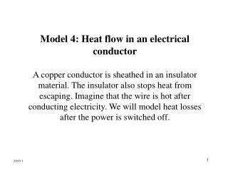
Model 4: Heat flow in an electrical conductor A copper conductor is sheathed in an insulator material. The insulator also stops heat from escaping. Imagine that the wire is hot after conducting electricity. We will model heat losses after the power is switched off. 2003/ 1. L. Copper

2003/ 1
E N D
Presentation Transcript
Model 4: Heat flow in an electrical conductorA copper conductor is sheathed in an insulator material. The insulator also stops heat from escaping. Imagine that the wire is hot after conducting electricity. We will model heat losses after the power is switched off. 2003/ 1
L Copper Insulation Step 1: Model and equationWe construct a simple heat flow model of the copper conductor of length L: figure 17: copper conductor • To describe the temperature from 0 to L we need: • an equation • The temperature at the boundaries. • The initial temperature. • Properties of the conductor material.
In any body heat will flow in the direction of decreasing temperature. The rate of flow is proportional to the gradient of the temperature: In one-dimension we can say: Rate of heat flow where u = temperature, K= thermal conductivity and A = cross-sectional area of the conductor. Because the wire is insulated heat only flows in the x-direction. We apply conservation of heat to a segment of the wire [x, x+dx]: Net change of heat in [x, x+dx] = Net flux of heat across boundaries + total heat generated in [x, x+dx]. Note: We assume that there is no heat generated within the body for this problem.
L Copper Insulation Flux of heat across the boundaries x x + Δx u(0,t)=0 u(L,t)=0 Extract the element between x and x + Δx: Rate of heat flowing into (or out of) back end Rate of heat flowing into (or out of) front end xx + Δx
The net heat transported into or out of this segment is the difference between the heat flux at front and back: Heat is produced as a consequence of electrical resistance. Imagine that we have left the power on and the conductor has heated up. When switched off the conductor will cool as heat is conducted out of the ends.
Rate of heat flowing into (or out of) back end Rate of heat flowing into (or out of) front end xx + Δx The total quantity of heat in the segment is: σρΔxAu, where σ = specific heatρ = density As it cools down we can say that the change in heat energy is:
Energy cannot be created so the sum of the heat leaving or entering through the ends added to the change in heat energy within the segment = 0We can write:Δheat energy + Δheat flux = 0 We can therefore write Δheat energy = -Δheat flux Rearrange:
If we letΔx→ 0, we get the 1 dimensional heat equation: x0
The expression K/σρ is called the diffusivity and is sometimes expressed as α2The 1 dim. heat equation is written: (27) (i.e. α2= K/σρ)
Step 2: General solutionWe can now produce a formula for the temperature along the wire if we can find a general form for the solution to the 1-dimensional equation. Instead of guessing we again use the method of “Separation of Variables”, making theassumption that the solution will be some function of x only multiplied by some function of t only: u = X(x)T(t)
Substitute the solution u=X(x)T(t) into the PDE: You get: Now separate variables (get everything that’s a function of x on one side and everything that’s a function of t on the other):
Both sides are equal to a constant. Call it k: We get the two equations:
Choose a sign for the constant that will give you sensible results: k= -2 You now get 2 differential equations:
Solutions to T and X are: (Demonstrate to yourself that these two expressions are solutions to the equations.)
The solution for u(x,t) equals T times X: or (28) This looks OK. There is an exponential ‘decay’ term for describing heat loss and the sinusoidal terms will be useful for fitting a solution within a fixed length as we will see. What form of solution would you get if you chose k= +2?
Step 3: Apply the boundary conditionsBoth ends were fixed at 0ºC.At x=0 0 1 To satisfy this b.c. we set E=0
At x=L We could make D=0 but this would not give us a useful solution. We therefore make sin(L) = 0 This will be zero for L= nπ, n=1,2,3… All the terms in the solution are given below:
Step 4: Satisfy the initial conditionsIf we know the initial temperature, we can find values for the constants Dn. Lets assume that the wire temperature was the same across the entire length of wire, say u(x,0)=T0.i.e. (30) Temperature at t=0: T0 x=0 x=L
To determine the Dn coefficients we again use a property of the sine function (Recall the guitar string model): if n=m (13) if nm
We multiply both sides of equation 30 by sin (mπx) and then integrate between the limits 0 and L. (30) All terms are equal to zero except when n =m.
Rearrange to find the value of the m’th term of the following equation: (15) Now we can evaluate Dm :
We now have an expression for our mth constant: Put this into the solution: (31)
I will show the solution to this problem in our class/tutorial. The following constants will be used for calculating the diffusivity of copper:Specific heat = 386 J/(kgC)Density = 8.96*103 kg/m3Thermal conductivity K = 385 J/(sec*meter*C).Therefore 2 = 1.11E-4 What are the units? Remember: α2= K/σρ
Assume L=0.1m and T0 = 100°C. I have used Microsoft Excel for this. The black line represents the sum of the 14 non-zero terms I have calculated. The blue line is the first term. Altogether I have plotted 5 of the non-zero terms. Solution at t=0
Solutions: t= 1 sec t= 10 sec