Download
1 / 58
580 likes | 725 Views
Algorithm Analysis & Sparse Vectors/Matrices & Recursion. Data Structures – Week #2. Outline. Performance of Algorithms Asymptotic Analysis Examples Exercises Sparse Vectors/Matrices Recursion Recurrences. Performance of Algorithms.

E N D
Algorithm Analysis & Sparse Vectors/Matrices & Recursion Data Structures – Week #2
Borahan Tümer Outline Performance of Algorithms Asymptotic Analysis Examples Exercises Sparse Vectors/Matrices Recursion Recurrences
Borahan Tümer Performance of Algorithms Algorithm: a finite sequence of instructions that the computer follows to solve a problem. Algorithms solving the same problem may perform differently. Depending on resource requirements an algorithm may be feasible or not. To find out whether or not an algorithm is usable or relatively better than another one solving the same problem, its resource requirements should be determined. The process of determining the resources of an algorithm is called algorithm analysis. Two essential resources, hence, performance criteria of algorithms are execution or running time memory space used. Given as a function of the algorithm's input size
Borahan Tümer Performance Assessment What we mean by the size of the input The number of elements in an array or linked list (e.g., for an algorithm that finds the highest value in a list) The size (dimensions) of a square (n × n) matrix. The length of a given fragment of text, etc. Problem: the algorithm (or rather, an implementation of it) can be run on different computers, with different clock speeds, different instruction sets, different memory access speeds, etc.? (not to mention different implementations) Instead of measuring actual time, we should measure something like number of operations that it takes to execute.
Borahan Tümer Assessment Tools We can use the concept the “growth rate or order of an algorithm” to assess both criteria. However, our main concern will be the execution time. We use asymptotic notations to symbolize the asymptotic running time of an algorithm in terms of the input size.
Borahan Tümer Asymptotic Notations We use asymptotic notations to symbolize the asymptotic running time of an algorithm in terms of the input size. The following notations are frequently used in algorithm analysis: O (Big Oh) Notation (asymptotic upper bound) Ω (Omega)Notation (asymptotic lower bound) Θ (Theta)Notation (asymptotic tight bound) o(little Oh) Notation (upper bound that is not asymptotically tight) ω(omega) Notation (lower bound that is not asymptotically tight) Goal: To find a function that asymptotically limits the execution time or the memory space of an algorithm.
Borahan Tümer Θ-Notation (“Theta”)Asymptotic Tight Bound Mathematically expressed, the “Theta” (Θ())concept is as follows: Let g: N->R* be an arbitrary function. Θ(g(n)) = {f: N->R* | (c1,c2R+)(n0N)(n n0) [0 c1g(n) f(n) c2g(n)]}, where R* is the set of nonnegative real numbers and R+ is the set of strictly positive real numbers (excluding 0).
Borahan Tümer Θ-Notation (“Theta”)Asymptotic Tight Bound
Borahan Tümer Θ-Notation by words Expressed by words; A function f(n) belongs to the set Θ(g(n)) if there exist positive real constants c1and c2(c1,c2R+) such that it can be sandwiched between c1g(n)andc2g(n) ([0 c1g(n) f(n) c2g(n)]),for sufficiently large n(n n0). In other words, Θ(g(n)) is the set of all functions f(n) tightly bounded below and above by a pair of positive real multiples of g(n), provided n is sufficiently large (greater than n0). g(n) denotes the asymptotic tight bound for the running time f(n) of an algorithm.
Borahan Tümer O-Notation (“Big Oh”)Asymptotic Upper Bound Mathematically expressed, the “Big Oh” (O())concept is as follows: Let g: N->R* be an arbitrary function. O(g(n)) = {f: N->R* | (c R+)(n0N)(n n0) [f(n) cg(n)]}, where R* is the set of nonnegative real numbers and R+ is the set of strictly positive real numbers (excluding 0).
Borahan Tümer O-Notation (“Big Oh”)Asymptotic Upper Bound
Borahan Tümer O-Notation by words Expressed by words; O(g(n)) is the set of all functions f(n) mapping (->) integers (N) to nonnegative real numbers (R*) such that (|) there exists a positive real constant c(c R+) and there exists an integer constant n0 (n0N) such that for all values of n greater than or equal to the constant (n n0), the function values of f(n) are less than or equal to the function values of g(n) multiplied by the constant c (f(n) cg(n)). In other words, O(g(n)) is the set of all functions f(n) bounded above by a positive real multiple of g(n), provided n is sufficiently large (greater than n0). g(n) denotes the asymptotic upper bound for the running time f(n) of an algorithm.
Borahan Tümer Ω-Notation (“Big-Omega”)Asymptotic Lower Bound Mathematically expressed, the “Omega” (Ω())concept is as follows: Let g: N->R* be an arbitrary function. Ω(g(n)) = f: N->R* | (c R+)(n0N)(n n0) [0 cg(n) f(n)]}, where R* is the set of nonnegative real numbers and R+ is the set of strictly positive real numbers (excluding 0).
Borahan Tümer Ω-Notation (“Big-Omega”)Asymptotic Lower Bound
Borahan Tümer Ω-Notation by words Expressed by words; A function f(n) belongs to the set Ω(g(n)) if there exists a positive real constant c(cR+) such that f(n) is less than or equal to cg(n) ([0 cg(n) f(n)]),for sufficiently large n(n n0). In other words, Ω(g(n)) is the set of all functions f(n) bounded below by a positive real multiple of g(n), provided n is sufficiently large (greater than n0). g(n) denotes the asymptotic lower bound for the running time f(n) of an algorithm.
Borahan Tümer Execution time of various structures Simple Statement O(1), executed within a constant amount of time irresponsive to any change in input size. Decision (if) structure if (condition) f(n) else g(n) O(if structure)=max(O(f(n)),O(g(n)) Sequence of Simple Statements O(1), since O(f1(n)++fs(n))=O(max(f1(n),,fs(n)))
Borahan Tümer Execution time of various structures O(f1(n)++fs(n))=O(max(f1(n),,fs(n))) ??? Proof: t(n) O(f1(n)++fs(n))t(n) c[f1(n)+…+fs(n)] sc*max [f1(n),…, fs(n)],sc another constant. t(n) O(max(f1(n),,fs(n))) Hence, hypothesis follows.
Borahan Tümer Execution Time of Loop Structures Loop structures’ execution time depends upon whether or not their index bounds are related to the input size. Assume n is the number of input records for (i=0; i<=n; i++) {statement block}, O(?) for (i=0; i<=m; i++) {statement block}, O(?)
Borahan Tümer Examples Find the execution time t(n) in terms of n! for (i=0; i<=n; i++) for (j=0; j<=n; j++) statement block; for (i=0; i<=n; i++) for (j=0; j<=i; j++) statement block; for (i=0; i<=n; i++) for (j=1; j<=n; j*=2) statement block;
Borahan Tümer Exercises Find the number of times the statement block is executed! for (i=0; i<=n; i++) for (j=1; j<=i; j*=2) statement block; for (i=1; i<=n; i*=3) for (j=1; j<=n; j*=2) statement block;
Borahan Tümer Recursion Definition: Recursion is a mathematical concept referring to programs or functions calling or using itself. A recursive function is a functional piece of code that invokes or calls itself.
Borahan Tümer Recursion Concept: A recursive function divides the problem into two conceptual pieces: a piece that the function knows how to solve (base case), a piece that is very similar to the original problem, hence still unknown how to solve by the function (call(s) of the function to itself).
Borahan Tümer Recursion… cont’d Base case: the simplest version of the problem that is not further reducible. The function actually knows how to solve this version of the problem. To make the recursion feasible, the latter piece must be slightly simpler.
Borahan Tümer Recursion Examples Towers of Hanoi Story: According to the legend, the life on the world will end when monks in a Far-Eastern temple move 64 disks stacked on a peg in a decreasing order in size to another peg. They are allowed to move one stack at a time and a larger disk can never be placed over a smaller one.
Borahan Tümer Towers of Hanoi… cont’d Algorithm: Hanoi(n,i,j) // moves n smallest rings from rod i to rod j F0A0 if (n > 0) { //moves top n-1 rings to intermediary rod (6-i-j) F0A2 Hanoi(n-1,i,6-i-j); //moves the bottom (nth largest) ring to rod j F0A5 move i to j // moves n-1 rings at rod 6-i-j to destination rod j F0A8 Hanoi(n-1,6-i-j,j); F0AB }
Borahan Tümer Towers of Hanoi… cont’d Example: Hanoi(4,i,j) 4 1 3 3 1 2 2 1 3 1 1 2 0 1 3 12 0 3 2 13 1 2 3 0 2 1 23 0 1 3 12 2 3 2 1 3 1 0 3 2 31 0 2 1 32 1 1 2 0 1 3 12 0 3 2 13 3 2 3 2 2 1 1 2 3 0 2 1 23 0 1 3 21 1 3 1 0 3 2 31 0 2 1 23 2 1 3 1 1 2 0 1 3 12 0 3 2 13 1 2 3 0 2 1 23 0 1 3
Towers of Hanoi… cont’d 4 1 3 start 3 1 2 start 2 1 3 start 1 1 2 start 1 2 3 end 2 1 3 end 2 3 2 start 1 3 1 start 1 1 2 end 1 2 3 start 12 13 23 12 3 1 2 end 2 3 2 end 1 1 2 end 3 2 3 start 2 2 1 start 1 2 3 start 1 2 3 end 1 3 1 end 1 1 2 start 31 32 12 13 23 2 2 1 end 1 3 1 end 1 3 1 start 2 1 3 start 1 1 2 start 1 1 2 end 1 2 3 start 21 31 23 12 13 23 4 1 3 end 3 2 3 end 2 1 3 end 1 2 3 end Borahan Tümer
Borahan Tümer Recursion Examples Fibonacci Series tn= tn-1 + tn-2; t0=0; t1=1 Algorithm long int fib(n) { if (n==0 || n==1) return n; else return fib(n-1)+fib(n-2); }
Fibonacci Series… cont’d • Tree of recursive function calls for fib(5) • Any problems??? Borahan Tümer
Borahan Tümer Fibonacci Series… cont’d Redundant function calls slow the execution down. A lookup table used to store the Fibonacci values already computed saves redundant function executions and speeds up the process. Homework: Write fib(n) with a lookup table!
Recurrences or Difference Equations • Homogeneous Recurrences • Consider a0tn + a1tn-1 + … + aktn-k = 0. • The recurrence • contains tivalues which we are looking for. • is a linear recurrence (i.e., tivalues appear alone, no powered values, divisions or products) • contains constant coefficients (i.e., ai). • is homogeneous (i.e., RHS of equation is 0). Borahan Tümer
Homogeneous Recurrences We are looking for solutions of the form: tn= xn Then, we can write the recurrence as a0 xn + a1xn-1+ … + ak xn-k = 0 • This kth degree equation is the characteristic equation (CE) of therecurrence. Borahan Tümer
Homogeneous Recurrences If ri, i=1,…, k,are k distinct roots of a0 xk + a1 xk-1+ … + ak = 0, then If ri, i=1,…, k,is a single root of multiplicity k, then Borahan Tümer
Borahan Tümer Inhomogeneous Recurrences Consider a0tn + a1tn-1 + … + aktn-k = bnp(n) where b is a constant; and p(n) is a polynomial in n of degree d.
Inhomogeneous Recurrences Generalized Solution for Recurrences Consider a general equation of the form (a0tn + a1tn-1 + … + aktn-k ) = b1np1(n) + b2n p2(n) + … We are looking for solutions of the form: tn= xn Then, we can write the recurrence as (a0 xk + a1 xk-1+ … + ak) (x-b1) d1+1 (x-b2) d2+1 …= 0; where diis the polynomial degree of polynomial pi(n). This is the characteristic equation (CE) of therecurrence. Borahan Tümer
Generalized Solution for Recurrences If ri, i=1,…, k, are k distinct roots of (a0 xk + a1 xk-1+ … + ak)=0 Borahan Tümer
Examples Homogeneous Recurrences Example 1. tn + 5tn-1 + 4 tn-2= 0; sol’ns of the form tn= xn xn + 5xn-1+ 4xn-2 = 0; n-2 trivial sol’ns (i.e., x1,...,n-2=0) (x2+5x+4) = 0; characteristic equation (CE) x1=-1; x2=-4; nontrivial sol’ns • tn= c1(-1)n+ c2(-4)n ; general sol’n Borahan Tümer
Borahan Tümer Examples Homogeneous Recurrence Example 2. tn-6 tn-1+12tn-2-8tn-3=0; tn= xn xn-6xn-1+12xn-2-8xn-3= 0; n-3 trivial sol’ns CE: (x3-6x2+12x-8) = (x-2)3= 0; by polynomial division x1= x2= x3 = 2; roots not distinct!!! tn= c12n+ c2n2n + c3n22n; general sol’n
Examples Homogeneous Recurrence Example 3. tn = tn-1+ tn-2; Fibonacci Series xn-xn-1-xn-2 = 0; CE: x2-x-1 = 0; ; distinctroots!!! ; general sol’n!! We find coefficients ciusing initial values t0 and t1 of Fibonacci series on the next slide!!! Borahan Tümer
Examples Example 3… cont’d We use as many tivalues as ci Check it out using t2!!! Borahan Tümer
Borahan Tümer Examples Example 3… cont’d What do n and tn represent? n is the location and tn the value of any Fibonacci number in the series.
Borahan Tümer Examples Example 4. tn = 2tn-1 - 2tn-2; n 2; t0 = 0; t1 = 1; CE: x2-2x+2 = 0; Complex roots: x1,2=1i As in differential equations, we represent the complex roots as a vector in polar coordinates by a combination of a real radius r and a complex argument : z=r*e i; Here, 1+i=2 * e(/4)i 1-i=2 * e(-/4)i
Borahan Tümer Examples Example 4… cont’d Solution: tn = c1 (2)n/2e(n/4)i+ c2 (2)n/2e(-n/4)i; From initial values t0 = 0, t1 = 1, tn = 2n/2sin(n/4); (prove that!!!)
Borahan Tümer Examples Inhomogeneous Recurrences Example 1. (From Example 3) We would like to know how many times fib(n) on page 22 is executed in terms of n. To find out: choose a barometer in fib(n); devise a formula to count up the number of times the barometer is executed.
Borahan Tümer Examples Example 1… cont’d In fib(n), the only statement is the if statement. Hence, if condition is chosen as the barometer. Suppose fib(n) takes tn time units to execute, where the barometer takes one time unit and the function calls fib(n-1) and fib(n-2), tn-1 and tn-2, respectively. Hence, the recurrence to solve is tn = tn-1 + tn-2 + 1
Examples Example 1… cont’d tn - tn-1 - tn-2 = 1; inhomogeneous recurrence The homogeneous part comes directly from Fibonacci Series example on page 33. RHS of recurrence is 1 which can be expressed as 1nx0. Then, from the equation on page 29, CE: (x2-x-1)(x-1) = 0; from page 30, Borahan Tümer
Examples Example 1… cont’d Now, we have to find c1,…,c3. Initial values: for both n=0 and n=1, if condition is checked once and no recursive calls are done. For n=2, if condition is checked once and recursive calls fib(1) and fib(0) are done. t0 = t1 = 1 and t2 = t0 + t1 + 1 = 3. Borahan Tümer
Examples Example 1… cont’d Here, tn provides the number of times the barometer is executed in terms of n. Practically, this number also gives the number of times fib(n) is called. Borahan Tümer
Borahan Tümer Sparse Vectors and Matrices In numerous applications, we may have to process vectors/matrices which mostly contain trivial information (i.e., most of their entries are zero!). This type of vectors/matrices are defined to be sparse. Storing sparse vectors/matrices as usual (e.g., matrices in a 2D array or a vector a regular 1D array) causes wasting memory space for storing trivial information. Example: What is the space requirement for a matrix mnxn with only non-trivial information in its diagonal if it is stored in a 2D array; in some other way? Your suggestions?
Borahan Tümer Sparse Vectors and Matrices This fact brings up the question: May the vector/matrix be stored in MM avoiding waste of memory space?