SCOPE Easy and Efficient Parallel Processing of Massive Data Sets
SCOPE Easy and Efficient Parallel Processing of Massive Data Sets. Adapted from a talk by : Sapna Jain & R. Gokilavani. Some slides taken from Jingren Zhou's talk on Scope : isg.ics.uci.edu/slides/MicrosoftSCOPE.pptx. Map-reduce framework.


SCOPE Easy and Efficient Parallel Processing of Massive Data Sets
E N D
Presentation Transcript
SCOPEEasy and Efficient Parallel Processing of Massive Data Sets Adapted from a talk by: Sapna Jain & R. Gokilavani Some slides taken from Jingren Zhou's talk on Scope : isg.ics.uci.edu/slides/MicrosoftSCOPE.pptx
Map-reduce framework • Good abstraction of group-by-aggregation operations • Map function -> grouping • Reduce function -> aggregation • Very rigid: Every computation has to be structured as a sequence of map-reduce pairs • Not completely transparent: users still have to use a parallel mindset • Lacks expressiveness of popular query language like SQL.
Scope • Structured Computations Optimized for Parallel Execution • A declarative scripting language • Easy to use: SQL-like syntax plus • Provides interfaces for customized operations • Users focus on problem solving as if on a single machine • System complexity and parallelism are hidden
Cosmos Storage System • Append-only distributed file system (immutable data store). • Extent is unit of data replication (similar to tablets). • Append from an application is not broken across extents. To make sure records are not broken across extents, application has to ensure record is not broken into multiple appends. • A unit of computation generally consumes a small number of collocated extents. /clickdata/search.log Append block Extent -2 Extent -1 Extent -0 Extent -3
Cosmos Execution Engine • A job is a DAG which consists of: • Vertices – processes • Edges – data flow between processes • Job manager schedules & coordinates vertex execution, fault tolerance and resource management. Map Map Map Reduce Reduce
Scope query language Compute the popular queries that have been requested at least 1000 times Scenario 1: SELECT query, COUNT(*) AS countFROM “search.log” USINGLogExtractorGROUP BY queryHAVING count> 1000ORDER BY count DESC; OUTPUTTO“qcount.result” Scenario 2: e = EXTRACT queryFROM “search.log” USINGLogExtractor; s1= SELECT query, COUNT(*) AS countFROMeGROUP BY query; s2 = SELECT query, countFROMs1 WHERE count> 1000; s3 = SELECT query, countFROMs2ORDER BY count DESC; OUTPUTs3TO “qcount.result” Data model: a relational rowset (set of rows) with well-defined schema.
Input and Output • EXTRACT : Constructs row from input data block. • OUTPUT : Writes row into output data block. • Built-in extractors and outputters for commonly used formats like text data & binary data. • User can write customized extractors and outputters for data coming from different sources. Presort is to tell system that rows on each vertex should be sorted before writing to disk. OUTPUT [<input> [PRESORT column [ASC|DESC] [, …]]]] TO <output_stream> [USING <Outputter> [(args)]] EXTRACT column[:<type>] [, …] FROM < input_stream(s) > USING <Extractor> [(args)] Defined schema of rows returned by extractor – used by compiler for type checking RequestedColumns is the columns requested in EXTRACT command publicclassLineitemExtractor : Extractor {public override Schema Produce(string[] requestedColumns, string[] args) { … } public overrideIEnumerable<Row> Extract(StreamReader reader, Row outputRow, string[] args) { … } } It is called once for each extent. Args is the arguments passed to extractor in EXTRACT statement.
Extract: Iterators using Yield Returns Greatly simplifies creation of iterators
SQL commands supported in Scope SELECT [DISTINCT] [TOP count] select_expression [AS <name>] [, …]FROM { <input stream(s)> USING <Extractor> | {<input> [<joined input> […]]} [, …] }[WHERE <predicate>][GROUP BY <grouping_columns> [, …] ][HAVING <predicate>][ORDER BY <select_list_item> [ASC | DESC] [, …]] joined input: <join_type> JOIN <input> [ON <equijoin>] join_type: [INNER | {LEFT | RIGHT | FULL} OUTER] • Supports different Agg functions: COUNT, COUNTIF, MIN, MAX, SUM, AVG, STDEV, VAR, FIRST, LAST. SQL commands not supported in Scope: • Sub-queries - but same functionality available because of outer join. • Non-equijoins : Non-equijoins require (n X m) replication of the two tables – which is very expensive (n & m is number of partitions of two tables).
Deep Integration with .NET (C#) • SCOPE supports C# expressions and built-in .NET functions/library R1 = SELECT A+C AS ac, B.Trim() AS B1FROM RWHEREStringOccurs(C, “xyz”) > 2#CSpublic static intStringOccurs(stringstr, string ptrn){ … }#ENDCS
User Defined Operators • Required to give more flexibility for advance users. • SCOPE supports three highly extensible commands: • PROCESS, • REDUCE, • COMBINE
Process • PROCESS command takes a rowset as input, processes each row, and outputs a sequence of rows • It can be used to provide un-nesting capability. • Another example: User wants to find all bigrams in the input document & create a row per bigram. PROCESS [<input>]USING <Processor> [ (args) ][PRODUCE column [, …]] publicclassMyProcessor: Processor { public override Schema Produce(string[] requestedColumns, string[] args, Schema inputSchema) { … } public overrideIEnumerable<Row> Process(RowSet input, Row outRow, string[] args) { … } }
Reduce • REDUCE command takes a groupedrowset, processes each group, and outputs zero, one, or multiple rows per group • Map/Reduce can be easily expressed by Process/Reduce • Example: User want to compute complex aggregation from a user session log (reduce on SessionId) but his computation may require data to be sorted on time within a session. REDUCE [<input> [PRESORT column [ASC|DESC] [, …]]]ONgrouping_column [, …] USING <Reducer> [ (args) ][PRODUCE column [, …]] Sort rows within the group on specific column (may not be reduce col). publicclassMyReducer: Reducer { public override Schema Produce(string[] requestedColumns, string[] args, Schema inputSchema) { … } public overrideIEnumerable<Row> Reduce(RowSet input, Row outRow, string[] args) { … } }
Combine COMBINE <input1> [AS <alias1>] [PRESORT …]WITH <input2> [AS <alias2>] [PRESORT …]ON <equality_predicate> USING <Combiner> [ (args) ]PRODUCE column [, …] • User define joiner • COMBINE command takes two matching input rowsets, combines them in some way, and outputs a sequence of rows • Example is multiset difference – compute the difference between 2 multisets (assume below S1 and S2 both have attributes A, B, C. COMBINE S1 WITH S2ON S1.A==S2.A AND S1.B==S2.B AND S1.C==S2.C USINGMultiSetDifferencePRODUCE A, B, C publicclassMyCombiner: Combiner { public override Schema Produce(string[] requestedColumns, string[] args, Schema leftSchema, string leftTable, Schema rightSchema, string rightTable) { … } public overrideIEnumerable<Row> Combine(RowSet left, RowSet right, Row outputRow, string[] args) { … } }
Importing Scripts • Similar to SQL table function. • Improves reusability and allows parameterization • Provides a security mechanism MyView.script: E = EXTRACT queryFROM@@logfile@@USINGLogExtractor ; EXPORT R = SELECT query, COUNT() AS countFROMEGROUP BY query HAVING count > @@limit@@; Query: Q1 = IMPORT “MyView.script”PARAMSlogfile=”Queries_Jan.log”,limit=1000; Q2 = IMPORT “MyView.script”PARAMSlogfile=”Queries_Feb.log”,limit=1000; …
Life of a SCOPE Query Scope Queries . . . Scope query Query output … … … Parse tree Parser / Compiler/ Security Optimizer . . . Physical execution plan Cosmos execution engine
Optimizer and Runtime Scope Queries(Logical Operator Trees) Logical Operators • SCOPE optimizer • Transformation-based optimizer • Reasons about plan properties (partitioning, grouping, sorting, etc.) • Chooses an optimal plan based on cost estimates • Vertex DAG: each vertex contains a pipeline of operators • SCOPE Runtime • Provides a rich class of composable physical operators • Operators are implemented using the iterator model • Executes a series of operators in a pipelined fashion Physical operators Cardinality Estimation Cost Estimation Optimization Rules Transformation Engine Optimal Query Plans(Vertex DAG)
Example – query count Extent-2 Extent-4 Extent-6 Extent-1 Extent-5 Extent-0 Extent-3 Extract Extract Extract Extract hash agg hash agg hash agg hash agg SELECT query, COUNT(*) AS countFROM “search.log” USINGLogExtractorGROUP BY queryHAVING count> 1000ORDER BY count DESC; OUTPUT TO “qcount.result” Compute partial count(query) on each machine Unlike Hyracks it does not execute vertices running on multiple machines in pipelined manner hash agg hash agg partition partition Hash partition on query Compute partial count(query) on a machine on a rack to reduce n/w traffic outside rack hash agg hash agg hash agg Filter rows with count > 1000 filter filter filter sort sort sort Sort merge for order by on count. Runs on a single vertex in pipelined manner. merge output Qcount.result
Scope optimizer • A transformation-based optimizer based on the Cascade framework (similar to volcano optimizer) • Generate all possible rewriting of query expression and chooses the one with lowest estimated cost. • Many of the traditional optimization rules from database systems are applicable, example: column pruning, predicate push down, pre-aggregation. • Need new rules to reason about partitioning and parallelism. • Goals: • Seamless generate both serial and parallel plans • Reasons about partitioning, sorting, grouping properties in a single uniform framework
Experimental results • Linear speed up with increase in cluster size. • Performance ratio = elapsed time / baseline • Data size kept constant. • Using log scale on performance ratio.
Experimental results • Linear scale up with data size. • Performance ratio = elapsed time / baseline. • Cluster size kept constant. • Using log scale on performance ratio.
Conclusions • SCOPE: a new scripting language for large-scale analysis • Strong resemblance to SQL: easy to learn and port existing applications • High-level declarative language • Implementation details (including parallelism, system complexity) are transparent to users • Allows sophisticated optimization • Future work • Multi-query optimization (with parallel properties, optimization opportunities have been increased). • Columnar storage & more efficient data placement.
Scope Vs. Hive • Hive is SQL like scripting language designed by Facebook – which works on Hadoop. • From, language constructs it is similar to Scope with few differences: • Hive does not allow user defined joiner (Combiner). Although it can be implemented as map & reduce extension by annotating row with tablename – but it is a bit hacky and non-efficient. • Hive provides support for user defined types in columns whereas Scope doesn’t. • Hive stores table serializer & de-serializer along with table metadata, user doesn’t have to specify Extractor in queries while reading the table (need to specify while creating the table). • Hive also provides for column oriented data storage using RCInputFileFormat. It give better compression and improve performance of queries which access few columns.
Scope Vs. Hive • Hive provides a richer data model – It partitions the table into multiple partitions & then each partition into buckets. ClickDataTable Partition ds=2010-02-02 Partition ds=2010-02-28 Bucket - 0 Bucket - 0 Bucket - n Bucket - n
Hive data model • Each bucket is a file in HDFS. The path of bucket will be: • <hive.warehouse.root.dir>/<tablename>/<partition key>/<bucketid> • <hive.warehouse.root.dir>/ClickDataTable/ds=2010-02-02/part-0000 • Table might not be partitioned: • <hive.warehouse.root.dir>/<tablename>/<bucketid> • Hierarchical partitioniningis allowed: • <hive.warehouse.root.dir>/ClickDataTable/ds=2010-02-02/hr-12/part-0000 • Hive stores partition column with metadata, not with data. That means a separate partition is created foreach value of partition column.
Scope Vs. Hive : Metastore Scope stores the output of query in unstructured data store. Hive also stores the output in unstructured HDFS but, it also stores all the metadata of the output table in a separate service called metastore. • Metastore uses traditional RDBMS as its storage engine because of low latency requirements. • The information in metastore is backed up regularly using replication server. • To reduce load on metastore – only compiler access metastore & pass all the information required during runtime in a xml file.
References • SCOPE: Easy and Efficient Parallel Processing of Massive Data SetsRonnie Chaiken, Bob Jenkins, Per-Ã…ke Larson, Bill Ramsey, Darren Shakib, Simon Weaver, and Jingren Zhou, VLDB 2008 • Hive - a petabyte scale data warehouse using Hadoop,A. Thusoo, J. S. Sarma, N. Jain, Shao Zheng, P. Chakka, Zhang Ning, S. Antony, Liu Hao, and R. Murthy, ICDE 2010 • Incorporating partitioning and parallel plans into the SCOPE optimizer. Jingren Zhou, Per-ÃkeLarson, Ronnie Chaiken, ICDE 2010
TPC-H Query 2 // Extract region, nation, supplier, partsupp, part … RNS_JOIN = SELECTs_suppkey, n_nameFROM region, nation, supplier WHEREr_regionkey == n_regionkeyANDn_nationkey == s_nationkey; RNSPS_JOIN = SELECTp_partkey, ps_supplycost, ps_suppkey, p_mfgr, n_nameFROM part, partsupp, rns_joinWHEREp_partkey == ps_partkeyANDs_suppkey == ps_suppkey; SUBQ = SELECTp_partkeyASsubq_partkey, MIN(ps_supplycost) ASmin_costFROMrnsps_joinGROUP BY p_partkey; RESULT = SELECTs_acctbal, s_name, p_partkey,p_mfgr, s_address, s_phone, s_commentFROMrnsps_joinAS lo, subqAS sq, supplier AS sWHERElo.p_partkey == sq.subq_partkeyANDlo.ps_supplycost == min_costANDlo.ps_suppkey == s.s_suppkeyORDERBYacctbalDESC, n_name, s_name, partkey; OUTPUTRESULT TO "tpchQ2.tbl";
Sub Execution Plan to TPCH Q2 • Join on suppkey • Partially aggregate at the rack level • Partition on group-by column • Fully aggregate • Partition on partkey • Merge corresponding partitions • Partition on partkey • Merge corresponding partitions • Perform join