Regression
Regression. Understanding relationships and predicting outcomes. Key concepts in understanding regression. The General Linear Model Prediction and errors in prediction Coefficients/weight Variance explained, variance not accounted for Effect of outliers Assumptions.

Regression
E N D
Presentation Transcript
Regression Understanding relationships and predicting outcomes
Key concepts in understanding regression • The General Linear Model • Prediction and errors in prediction • Coefficients/weight • Variance explained, variance not accounted for • Effect of outliers • Assumptions
Relations among variables • A goal of science is prediction and explanation of phenomena • In order to do so we must find events that are related in some way such that knowledge about one will lead to knowledge about the other • In psychology we seek to understand the relationship among variables that are indicators of an innumerable amount of information about human nature in order better understand ourselves and why we are the way we are
Before getting too far • While we are getting ‘mathy’ in our discussion of regression, there’s no way around it. All the analyses you see in articles are ‘simply’ mathematical models fit to the data collected. Without an understanding of that aspect on some level, there is no way to do or understand psychological science in any meaningful way. • However it is important to remember why we are doing this. • Stats, as a reminder, is simply a tool. Our primary interest however is in understanding human behavior, and potentially the underlying causes of it. • We are interested in predicting what causes physical and emotional pain, individual happiness, how the mind works, how and why we make the choices we do and so on. • So to aid you in your own understanding, before going on, pick a simple relationship between two variables you would be interested in, and keep them ‘in mind’ as we go through the following • Identify one as the predictor, one as the outcome. Write them down and refer to them as we go along.
Correlation • While we could just use our N of 1 personal experience to try and understand human behavior, a scientific (and better) means of understanding the relationship between variables is by means of assessing correlation • Two variables take on different values, but if they are related in some fashion they will covary • They may do so in a way in which their values tend to move in the same direction, or they may tend to move in opposite directions • The underlying statistic assessing this is covariance, which is at the heart of every statistical procedure you are likely to use inferentially
Covariance and Correlation • Covariance as a statistical construct is unbounded and thus difficult to interpret in its raw form • Correlation (Pearson’s r) is a measure of the direction and degree of a linear association between two variables • Correlation is the standardized covariance between two variables
Regression • Regression allows us to use the information about covariance to make predictions • Given knowledge regarding the value of one variable, we can predict an outcome with some level of accuracy • The basic model is that of a straight line (the General Linear Model) • The formula for a straight line is: • Y = bX + a • Y = the calculated value for the variable on the vertical axis • a = the intercept, where the line crosses the Y axis • b = the slope of the line • X = values for the variable on the horizontal axis • Only one possible straight line can be drawn once the slope and intercept are specified, and once this line is specified, we can calculate the corresponding value of Y for any value of X entered • In more general terms Y = Xb + e, where these elements represent vectors and/or matrices (of the outcome, data, coefficients and error respectively), is the general linear model to which most of the techniques in psychological research adhere to
The Line of Best Fit • Real data do not conform perfectly to a straight line • The best fit straight line is that which minimizes the amount of variation in data points from the line • The common approach, but by no means the only or only acceptable method, attempts to derive a least squares regression line which minimizes the squared deviations of the points from it • The equation for this line can be used to predict or estimate an individual’s score on some outcome on the basis of his or her score on the predictor • Y-hat here is the predicted (fitted) value for the DV, not the actual value of the DV for a case1
Variable X A Criterion Variable Y B C Variable Z Least Squares Modeling • When the relation between variables are expressed in this manner, we call the relevant equation(s) mathematical models, and they reflect our theoretical models • The intercept and weight values are called the parameters of the model • While typical regression analysis by itself does not determine causal relations, the assumption indicated by such a model is that the variable on the left-hand side of the previous equation is being caused by the variable(s) on the right side • The arrows explicitly go from the predictors to the outcome, not vice versa1
Parameter Estimation Example • Let’s assume that we believe there is a linear relationship between X and Y. • Which set of parameter values will bring us closest to representing the data accurately?
Estimation Example • We begin by picking some values, plugging them into the equation, and seeing how well the implied values correspond to the observed values • We can quantify what we mean by “how well” by examining the difference between the model-implied Y and the actual Y value • This difference between our observed value and the one predicted, , is often called error in prediction, or the residual • The residual Sum of Squares here is 160
Estimation Example • Let’s try a different value of b, i.e. a different coefficient, and see what happens • Now the implied values of Y are getting closer to the actual values of Y, but we’re still off by quite a bit
Estimation Example Things are getting better, but certainly things could improve
Estimation Example Getting better still
Estimation Example • Now we’ve got it • There is a perfect correspondence between the predicted values of Y and the actual values of Y • No residual variance • Also no chance of it ever happening with real data
Estimates of the constant and coefficient in the simple setting • Estimating the slope of the line: • This is our regression coefficient, and it represents the amount of change in the outcome seen with 1 unit change in the predictor. It requires first estimating the covariance • Estimating the Y intercept • where and are the means based on the sets of the Y and X values respectively, and b is the estimated slope of the line • These calculations ensure that the regression line passes through the point on the scatterplot defined by the two means
Break time • Stop and look at your chosen variables of interest. • Write down our general linear model1, but substituting the your predictor and outcome for the X and Y respectively • Do you understand how the measurable relationship between the two comes into play? • Can you understand the slope in terms of your predictor and its effect on the outcome? • Can you understand the intercept in terms of a pictorial relationship of this model? • Can you understand the notion of a ‘fitted’ value with regard to your outcome? • If you’re okay at this point, it’s time to see how good a job we’re doing in this prediction business
Breaking Down the Variance • Total variability in the dependent variable (i.e. how the values bounce about the mean) comes from two sources • Variability predicted by the model i.e. what variability in the dependent variable is due to the predictor • How far off our predicted values are from the mean of Y • Error or residual variability i.e. variability not explained by the predictor variable • The difference between the predicted values and the observed values Total variance = predicted variance + error variance
Regression and Variance • It’s important to understand this conceptually in terms of the variance in the DV we are trying to account for • With perfect prediction, we’d have zero residual variance, all variance in the outcome variable is accounted for • With zero prediction, all variance would be residual variance • Essentially the same as ‘predicting’ the mean each time • Note that if we knew nothing else, that’s all we could predict • The fact that there is a correlation between the two allows us to do better • No correlation, no fit
R² = variance of predicted values divided by the total variance of observed DV values R2 is also the square of the correlation between those fitted values and the original DV R2: the coefficient of determination • The square of the correlation, R², is the fraction of the variation in the values of the outcome that is explained by our predictor • We can show this graphically using a Venn diagram • R2 = the proportion of variability shared by two variables (X and Y) • The larger the area of overlap, the greater the strength of the association between the two variables
Measures of ‘fit’ • Many measures of fit are available, though with regression you will typically see (adjusted) R2 • Some others include: • Proportional improvement in prediction (as seen in Howell) • From path analysis/sem literature: • Χ2 (typically a poor approach as we have to ‘accept the null’) • GFI (goodness of fit index) • AIC (Akike information criterion) • BIC (Bayesian information criterion) • Some of these, e.g. the BIC, have little utility except in terms of model comparison • One of the means of getting around NHST is changing our question from ‘Is it significant?’ to ‘Which model is better?’
The Accuracy of Prediction • How else might we measure model fit? • The error associated with a prediction (of a Y value from a known X value) is a function of the deviations of Y about the predicted point • The standard error of estimate1 provides an assessment of accuracy of prediction • The standard deviation of Y predicted from X • In terms of R2, we can see that the more variance we account for the smaller our standard error of estimate will be
Example Output • Study hours predicted by Book cost1 • Assumption is greater cost is indicative of more classes and/or required reading • Given just the df and sums of squares, you should be able to fill out the rest of the ANOVA summary table save the p-value • Given the coefficient and standard error, you should be able to calculate the t • Note the relationship of the t-statistic and p-value for the predictor and the F statistic and p-value for the model • Notice the small coefficient? What does this mean? • Think of the Book Cost scale and the Hours study per day • A one unit movement in Book Cost is only a dollar, and corresponds to .0037 hours. • With a more meaningful increase in 100 dollars, we can expect study time to increase .37 hours, or about 22 minutes per day
Interpreting regression: Summary of the Basics • Intercept • Value of the outcome when the predictor value is 0 • Often not meaningful, particularly if it’s practically impossible to have a value of 0 for a predictor (e.g. weight) • Slope • Amount of change in the outcome seen with 1 unit change in the predictor • Standardized regression coefficient • Amount of change in the outcome seen in standard deviation units with 1 standard deviation unit change in the predictor • In simple regression it is equivalent to the Pearson r for the two variables • Standard error of estimate • Gives a measure of the accuracy of prediction • R2 • Proportion of variance explained by the model
Other things to consider • The mean of the predicted values equals the mean of the original DV • The regression line passes through the point representing the mean of both variables • In tests of significance, we can expect sample size, scatter of points about the regression line, and range of predictor values to all have an effect • Coefficients can be of the same size but statistical significance and SSreg will vary (different standard errors)
Hold on a second… • And you thought we were finished! • In order to test for model adequacy, we have to run the regression first. • So yes, we are just getting started. • The next notes refer to testing the integrity of the model in simple regression, but know there are many more issues once additional predictors are added (i.e. the usual case)

