Basic Probability
Basic Probability. Frequency Theory. A mathematical approach to making the notion of “chance” rigorous. Best applied to processes which can be repeated many times , independently , and under the same conditions . Coin tossing Dice rolling (craps) Card games (blackjack, poker, etc.).

Basic Probability
E N D
Presentation Transcript
Frequency Theory • A mathematical approach to making the notion of “chance” rigorous. • Best applied to processes which can be repeated many times, independently, and under the same conditions. • Coin tossing • Dice rolling (craps) • Card games (blackjack, poker, etc.)
Probability • The probability of an event is the percentage of the time it is expected to happen if the process is repeated many times, independently and under the same conditions. • If a fair coin is tossed, P(heads) = 0.5 or 50%, and P(tails)=0.5. • This means: if we toss a fair coin 1000 times, we expect to get about 500 heads. • If a fair six-sided die is rolled, P(rolling a 4)= 0.1667 or 16.67% • This means: if we roll a fair die 6000 times, we expect to roll a 4 about 1000 times.
A few basic facts • Probabilities must be between 0 and 1 (0% and 100%) • Impossible events have probability 0. • Events sure to happen have probability 1. • The probability of an event is 1 minus the probability of the opposite event. P(rolling a number less than 6) = 1 – P(rolling a 6) = 1 - .
Canonical Example • A box contains three tickets, labeled “1”, “2”, and “3”. If you choose one ticket at random, what is the probability that you draw the ticket labeled “3”? • “At random” means each ticket has an equal chance of being drawn. • P(drawing ticket “3”) = • This means: If everyone in the room had identical boxes of three tickets, about one third of the people would draw ticket “3”.
Canonical Example • A box contains three tickets, labeled “1”, “2”, and “3”. If you choose one ticket at random, what is the probability that you draw the ticket labeled “3”? • “At random” means each ticket has an equal chance of being drawn. • P(drawing ticket “3”) = • What if the box contains 30 tickets: 10 tickets labeled “1”, 10 labeled “2”, and 10 labeled “3”?
Canonical Example • If you choose two tickets at random, what is the probability that both are labeled “3”? • The answer depends on whether or not you replace the first ticket you draw. • However, the math you use to find the answer does not.
Multiplication Rule • The probability that two events will both happen equals the probability of the first event multiplied by the probability of the second event given that the first event happened. P( A and B ) = P( A ) x P( B given A ) • The probability P( B given A ) is called a conditional probability. It’s sometimes written P( B | A ).
Drawing without replacement • In the example above, suppose you choose tickets without replacement. • The probability of getting a “3” on the first draw is . • If you get a “3” on the first draw, there are only 9 tickets remaining labeled “3”. Thus your chances of getting a “3” on the second draw given you drew a 3 on the first draw are . • The probability of drawing two “3”s without replacement is .
Drawing with replacement • Now suppose you draw two tickets at random, but you replace the first ticket you drew. • The probability of getting a “3” on the first draw is still • The probability of getting a “3” on the second draw given that you drew a “3” on the first draw is also because you replaced the ticket you drew. • Thus the probability of drawing two “3”s with replacement is
Independence • Two events are said to be independent if the probability of the second event does not depend on the outcome of the first event. • That is, if P( B given A ) = P( B ) • When drawing tickets at random with replacement, the draws are independent. • Without replacement, the draws are dependent.
Examples • A fair coin is tossed twice. If the second toss is heads, you win a dollar. • If the first toss is heads, what is your chance of winning a dollar? • If the first toss is tails, what is your chance of winning a dollar? • The events “first toss is heads” and “second toss is heads” are independent.
Examples • Two cards are dealt off the top of a well-shuffled deck of 52 standard playing cards. • What is the probability that the second card is the queen of hearts? • What is the probability that the second card is the queen of hearts given that the first card is a spade? • The events “drawing the queen of hearts” and “drawing a spade” are dependent.
Warnings • Use caution when multiplying probabilities. In general, P( A and B ) = P( A ) x P( B given A ). Only if A and B are independent is it true that P( A and B ) = P( A ) x P( B ). • Don’t apply the theory outlined above to unique events – events that can’t be repeated many times, independently and under the same conditions. • What is the probability that tomorrow’s high temperature is 73 degrees Fahrenheit?
Activity: The Law of Averages • Perform 50 coin flips. • For each flip, if the coin lands with “heads” showing, record a “1”. If “tails” is showing, record a “0”. • Bring me the following data: • The total number of heads • The longest “run” of heads or tails • The number of runs of 4 heads (Note: a run of 5 heads = 2 runs of 4, a run of 6 heads = 3 runs of 4, etc.) • The number of times a head followed a run of 4 heads • Number of heads before the first tail. • Number of heads after the last tail.
John Kerrich’s results In first 2000 tosses, there were 130 runs of 4 heads. In 69 cases the run was followed by a head, in 61 cases, it was followed by a tail.
Key takeaway points • As the number of tosses increases, so does |(# heads) – (expected # of heads)| but the percentage difference decreases. • The number of heads differs from the expected number due to chance variability. • If the experiment is repeated, the number of heads is likely to be different. • Runs don’t change the probability of the next toss. (Tosses are independent events.)
Modeling Chance Processes • How many heads do you get if you toss a coin many times? • How much money does a casino make on roulette? • How accurate is a sample survey? These questions are about chance processes.
Box Models • General strategy for analyzing chance processes: • Find an analogy between the process you’re interested in and drawing numbers at random from a box. • Connect the variability you want to know about with the chance variability in the sum of the numbers drawn.
Box Models • Three key questions • What numbers go into the box? • How many of each number? • How many draws?
Box models for Roulette • Example 1: Betting $1 on red. • Numbers in the box: +1, -1 (win pays even money) • How many of each: 18 tickets: +1, 20 tickets: -1 • Number of draws: the number of plays • We draw at random, with replacement • The sum of the draws is your net gain. • Ten plays: R R R B G R R B B R • Ten draws: +1 +1 +1 -1 -1 +1 +1 -1 -1 +1 • Net gain: +2
Box models for Roulette • Example 2: Betting $1 on a single number • Numbers in the box: +35, -1 (win pays 35 to 1) • How many of each: 1 ticket: +35, 37 tickets: -1 • Number of draws: number of plays • We draw with replacement.
A box model in statistics • A political candidate wants to enter a primary in a district with 100,000 eligible voters, but only if he has a good chance of winning. He hires a survey organization which samples 2500 voters. In the sample, 1328 favor the candidate. How far off is the survey likely to be? • Numbers in the box: 1 (vote for), 0 (vote against) • How many of each: unknown, 100,000 total • Number of draws: 2500 • We draw without replacement. • Sum of draws: number of votes for the candidate (1328)
Expected Value • The outputs of a chance process vary around the expected value. • Drawing with replacement, the expected value for the sum of draws from a box is EV= (number of draws) x (average of numbers in box) • Example: The expected value of betting $1 on red 10 times in roulette is 10 x If we made 100 bets, the expected value would be about -$5.30
Expected Value • What is the expected value of betting $1 on the number 7 ten times? • The box has 1 ticket of $35 and 37 tickets of -$1. The average of numbers in the box is • Thus the expected value of betting on 7 ten times is the same: about -$0.53
Standard Error • The standard error(SE) for the sum of draws measures the expected amount of chance error. • Drawing randomly with replacement from a box, SE for sum = (SD of numbers in box) • As the number of draws increases, so does the error. But the percent error decreases. % error =
Standard Error • What is the standard error for number of heads in 100 tosses of a fair coin? • Write down the box model. • The SD of the numbers in the box is (short-cut for lists of two values) • The SE for the sum is thus • For 1400 tosses, the SE for the sum is
Standard Error • Example: Betting $1 on red in roulette 10 times. • The SD of the box is • The standard error for the sum of draws is thus SE for sum • So while the expected value is -$0.53, it is likely that the actual value will be off by up to $3.16. • If we make the bet 100 times, the SE is $9.99.
Standard Error • When drawing without replacement, the formula for SE includes the correction factor • We then have SE without replacement = (SE with replacement) x (correction factor) • More on this situation in a few weeks.
Activity: Gettysburg Address • Choose 10 words at random (or, as randomly as you can) from the Gettysburg Address. • Record the mean word length. • Choose 20 words at random and record the mean word length (to one decimal place). (Think of this as drawing from a box where tickets are labeled with word lengths.)
Probability Histograms And the Central Limit Theorem
Probability Histogram • A graph representing the probability of each numerical outcome in a chance process. • Rectangles have width 1 and are centered on a possible outcome. • The area of each rectangle is the probability of the corresponding outcome. • Based on chance (theory) not on observations
Examples • Two dice are rolled and their sum is recorded.
Examples • Two dice are rolled and their sum is recorded.
Examples • Two dice are rolled and their sum is recorded. • Two dice are rolled and their product is recorded.
Probability vs. Density Histogram • Example: Roll two dice and record the sum. • Probability histogram
Probability vs. Density Histogram • Example: Roll two dice and record the sum. • Probability histogram • Repeat the experiment several times and make a density histogram of the results. (http://www.stat.sc.edu/~west/javahtml/CLT.html)
Probability vs. Density Histogram • If the number of repetitions is large enough, Density histogram Probability histogram • This does not depend on the shape of the probability histogram.
Probability vs. Density Histogram One hundred random selections of a single word from the Gettysburg Address
Normal Approximation • A major achievement of 18th century mathematics was de Moivre’s proof that the probability histogram for the number of heads in N coin tosses follows the normal curve very closely for large values of N.
Central Limit Theorem • When drawing at random with replacement from a box, the probability histogram for the sum of the draws or mean of the draws will follow the normal curve, even if the contents of the box do not.
Central Limit Theorem • When drawing at random with replacement from a box, the probability histogram for the sum of the draws or mean of the draws will follow the normal curve, even if the contents of the box do not. • The number of draws must be reasonably large. What “reasonably large” means does depend on the contents of the box. • To match the normal curve, you must convert to z-values using E.V. and S.E.
Central Limit Theorem • The probability histogram for the product of the draws will not follow the normal curve.