Download

1 / 19
190 likes | 209 Views
This article explores the kernelization technique for the maximum leaf spanning tree problem with positive vertex weights, including its complexity, parameterized complexity, and improved running times and kernel sizes. It also introduces the weighted version of the problem and provides a kernelization strategy.

E N D
Bart JansenKernelization for Maximum Leaf Spanning Tree with Positive Vertex Weights CIAC 2010, Rome
Maximum Leaf Spanning Tree • Max Leaf • Input: Connected graph G, integer k • Question: Does G have a spanning tree with at least k leaves? • Applications in Network Design, Facility Location • Strongly related to Connected Dominating Set • Spanning tree ≥ k leaves Connected dominating set ≤ n – k
Fixed-Parameter Tractability • Solve NP-hard problems exactly • Measure the structure of an instance through a parameter, and determine whether combinatorial explosion can be restricted to the parameter • Example: Vertex Cover • “Does graph G have a vertex cover of size k?” • Use the requested size k as the parameter • Problem can be solved in O(2kn2) time • General case: • instance of a parameterized problem is a tuple (x,k) where x is the “classical” instance and k measures some property of x • Problem is Fixed Parameter Tractable (FPT) if it can be solved in f(k)|x|c time for a computable function f and constant c
Kernelization • Kernelization is a technique to obtain FPT algorithms, and is useful in a broad context for preprocessing • A kernelization algorithm (or kernel) for a parameterized problem is a polynomial-time algorithm that transforms (x,k) into (x’,k’) such that: • (x,k) and (x’,k’) are equivalent instances of the same problem • |x’|, k’ ≤ f(k) for some computable function f • The function f is the size of the kernel • Intuitively: a kernelization uses polynomial time to obtain an equivalent instance whose size depends only on the old parameter k, but not on the old instance size • Example: Vertex Cover • We can transform (G,k) into (G’,k’) such that |V’| ≤ 2k • Size of kernel is O(k2)
Parameterized Complexity of Max Leaf • Use the target number of leaves k as the parameter • Long history of improved running times and kernel sizes • Current best: • Max Leaf is tractable from the parameterized perspective • We should see which generalizations are tractable! • Introduce vertex weights
Weighted Maximum Leaf Spanning Tree • Weighted Max Leaf • Input: Connected graph G with vertex weights, value k • Question: Does G have a spanning tree whose leaves have combined weight at least k? • Parameter:k • Complexity of the problem depends on allowed weights • Our results: Weight 11 Weight 11 Weight 16
Leafy Spanning Trees • Let G be a connected graph on n vertices such that: • The graph is not a simple cycle • No degree-1 vertex is adjacent to a degree-2 vertex • There is no path of ≥ 4 consecutive degree-2 vertices • Then G has a spanning tree with n/7.5 leaves • Every leaf has weight ≥ 1 G has a S.T. with weight n/7.5
Kernelization strategy • Transform G into a graph G’ that satisfies the given 3 properties, such that MaxWeight(G) = MaxWeight(G’) • Then: • MaxWeight(G’) ≥ MaxLeaves(G’) ≥ |V’|/7.5 |V’| ≤ 7.5 ∙ MaxWeight(G’) • Kernelization algorithm transforms (G,k) into (G’,k) in polynomial time • If |V’| ≥ 7.5k then output YES • Otherwise |V’| < 7.5k, output (G,k’)
Rule 1: Solve cycles • A spanning tree for a cycle avoids exactly 1 edge • Choose an edge with maximum weight of its endpoints and delete it
Rule 2: Shrink pendant paths • Any spanning tree must use all edges on a degree-2 path to a leaf • We can delete the degree-2 vertices and re-attach the leaf
Rule 3: Shrink large path components • Consider a path component of degree-2 vertices between x,y of degree ≠ 2 • A spanning tree avoids at most one edge in this component • When avoiding an edge not incident on x or y, it’s optimal to avoid one with maximum weight of its endpoints • Reduce by merging all degree-2 vertices except the first and last into one • Set weight to: maximum edge weight – max(first,last)
Better Bounds • If additionally: • Distinct degree-2 vertices have distinct open neighborhoods • Every triangle {x,y,z} contains a vertex of degree ≥ 4 • Then G has a spanning tree with n/5.5 leaves • Gives kernel with 5.5k vertices
Proof of the extremal result • Extends a technique of Griggs, Kleitman and Shastri who showed: • every cubic graph on n vertices has a spanning tree with n/4 leaves • Amortized analysis by “keeping track of dead leaves” • Constructive proof • Initialize a tree T subgraph as a star around 1 vertex • As long as T does not span G: show we can augment to a bigger tree T’ • Show that the increase in # vertices is balanced against the increase in # leaves • Prove that as long as the tree does not span G, some augmentation is possible • Extensive case analysis to get to n/5.5 • Factor 5.5 is best-possible for these graphs
Kernelization result • [Decision version] Given an instance (G,k) of Weighted Max Leaf with weights ≥ 1, we can compute in O(n+m) time an equivalent instance (G’,k’) such that: • G has a spanning tree with weight ≥ k G’ has a spanning tree with weight ≥ k’, • |V’| ≤ 5.5k’, • k’ ≤ k. • [Optimization version] Given an instance G of Weighted Max Leaf with weights ≥ 1, we can compute in O(n+m) time an instance G’ and constant c such that: • opt(G) = opt(G’) + c, • |V’| ≤ 5.5 opt(G’) • c ≥ 0.
Approximability • Through reduction from Independent Set we obtain results on approximability of Weighted Max Leaf with weights ≥ 1 • No n1/2-ε approximation • No OPT1/3-ε approximation in polynomial time for any ε > 0 unless P=NP • Surprising behavior • linear-vertex kernel butno constant-factor approximation • For weights in the range [1..c] there is a 2c approximation
Conclusion • We should study generalizations of FPT problems • Eliminating long degree-2 paths guarantees MaxLeaves ≥ |V|/c • Weighted Max Leaf with weights ≥ 1 has a kernel with 5.5k vertices by using weight-aware reduction rules • Other results • Weighted Max Leaf with all weights 0 or ≥ 1 has a linear-vertex kernel on bounded-genus graphs • Open problems • Is there a fast FPT algorithm for Weighted Max Leaf? • Are there other FPT problems that remain tractable when allowing vertex weights? • What is the effect of vertex weights on kernelizability?