Download
1 / 19
190 likes | 294 Views
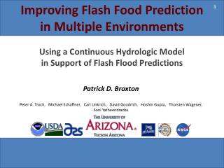
This study focuses on improving flash flood prediction using a continuous hydrologic model across various environments. The research addresses the unique catchment capabilities to absorb precipitation while examining the influences of high potential evapotranspiration, precipitation variations, and snow dynamics. Conducted in both humid and semi-arid watersheds in New York's Catskill Mountains and southeastern Arizona, this investigation integrates advanced methodologies to understand extreme streamflow events, thus enhancing the reliability of flood predictions.

E N D
1 Improving Flash Food Prediction in Multiple Environments Patrick D. Broxton Peter A. Troch, Michael Schaffner, Carl Unkrich, David Goodrich, Hoshin Gupta, Thorsten Wagener, Soni Yatheendradas Using a Continuous Hydrologic Model in Support of Flash Flood Predictions
Motivation: Considerations for Modeling Extreme Streamflow Events • What is a catchment’s ability to absorb precipitation? High Potential ET Warm Precipitation Wet Dry Less Water in Storage More Water in Storage Cool Runoff Infiltration Low Potential ET Baseflow
Motivation: Considerations for Modeling Extreme Streamflow Events • What is the “true” precipitation input? Rain Gauges Radar Satellite Observations More Accurate Less Accurate Less Coverage More Coverage Large Scale Small Scale • What about Snow?
4 SM-hsB Overview ET Soil Moisture – hillslope Bousinesq Model Infiltration Land Surface Module Subsurface Module • Water and energy balance at the land surface • Root zone water balance • Incorporates Snow • Lateral transport of soil water Root Zone Transmission Zone hsB Aquifer Deep Aquifer 1) Keep track of the hydrologic state between flood model runs 2) Distributed so that it can account for spatial variability of terrain and atmospheric forcing
5 Study Sites
6 Study Sites – New York Watersheds • Five watersheds in New York’s Catskill Mountains: • Humid catchments that are focus of current efforts a) W. Branch Delaware River (332 sq mi) b) W. Branch Delaware River (134 sq mi) c) Platte Kill (35 sq mi) d) East Brook (25 sq mi) e) Town Brook (14 sq mi)
Study Sites – Arizona Watersheds 7 • Three watersheds in southeastern Arizona: • Semi-arid catchments to compliment humid catchments a) Sabino Canyon (35.5 sq mi) b) Rincon Creek (44.8 sq mi) c) Walnut Gulch (57.7 sq mi)
Hydrology of New York Watersheds 8 New York Basins Arizona Basins 1.6 Runoff Coefficient (Q/P) Delaware River (Walton) Delaware River (Delhi) East Brook 1.2 PRISM – Average Yearly Precipitation (mm) Runoff Coefficient (Q/P) Town Brook Sabino Canyon 0.8 Plate Kill Rincon Creek 0.8 900 Walnut Gulch 31.8 0.6 800 Latitude (degrees) 0.4 700 32 0.4 600 0 0.2 32.2 May 500 Mar Aug Nov Apr Jun Jan Feb Sep Oct Dec Jul 1200 42.2 400 Month Latitude (degrees) 32.4 0 1150 May Mar Aug Nov 300 Apr Jun Jan Feb Sep Oct Dec Jul -111 -110.6 -110.2 -109.8 42.3 Month 1100 Longitude (degrees) 42.4 1050 42.5 75.2 -75 -74.8 -74.6 Longitude (degrees) Date
9 Modeling with SM-hsB
Land Surface Module - Overview 10 Atmospheric Inputs: Shortwave Radiation Longwave Radiation Precipitation Temperature Pressure Humidity Wet Canopy Evaporation/ Snow Interception Trees Precipitation Long Wave Radiation Infiltration/Runoff Shortwave Radiation Wintertime Snowpack Variable Canopy Cover Near-Surface Soil Layer Stream Fully distributed, runs on hourly timesteps (diurnal cycle is important) Based on energy balance principles – similar to Utah Energy Balance Model
Land Surface Module - Calibration 11 Can be run at a point: e.g. Calibrate to a point measurement such as a snow pillow ...or over an area: e.g. Calibrate over an area to remotely sensed data or to a data assimilation system Photo courtesy Jim Porter at NYCDEP 140 R2 = 0.81 Over a multi-year span, it is generally tuned to compare well with SNODAS, but for specific years, it can be refined using other measurements 120 SM-hsB SWE (mm) 100 80 SWE (mm) 60 40 120 20 120 0 80 80 0 20 40 60 80 100 120 140 40 40 SNODAS SWE (mm) 0 0 1/1/2008 4/1/2008 1/1/2007 4/1/2007
Land Surface Module - Simulation 12 Preliminary results for 2009-2010 Snow Season in W. Branch Delaware River Watershed All precipitation inputs are derived from the MPE SWE (mm) 200 January 15,2010 160 100 mm 120 80 50 mm 40 0 12/1/2009 1/1/2010 2/1/2010 3/1/2010 4/1/2010 Date 0 January 25,2010 February 15,2010 February 28,2010
Subsurface Module - Overview 13 Root Zone Water Balance / Baseflow ET Infiltration Runoff Root Zone Streamflow Routing Transmission Zone hsB Aq. Baseflow hsB Aquifer Deep Aquifer Deep Aq. Baseflow Semi distributed, runs on daily or hourly timesteps
Subsurface Module - Calibration 14 Calibration procedure relies on a baseflow separation Portions of the model are reconstructed from the steamflow signatures (hydrology backwards) Log(Streamflow-mm) 2 70 Streamflow/Baseflow/Runoff (mm) Streamflow Baseflow HSB Aquifer 1 60 Runoff 50 0 Deep Aquifer 40 -1 30 0 5 10 15 35 20 25 30 Effective Time (days) 20 Calibration procedure based on that developed by Gustavo Carrillo and Peter Troch at the University of Arizona 10 0 1/1/2005 4/2/2006 7/3/2007 10/1/2008 12/31/2009 Date
Subsurface Module - Simulation 15 Simulation for Delaware River (Walton) using MPE as input log(Streamflow – mm/day) Baseflow (mm/day) Data 1 Normalized Streamflow Generation 20 Model Model 101 15 0.8 Data 0.6 10 100 0.4 5 Data Model 0.2 0 10-1 1/1/2005 4/2/2006 7/3/2007 10/1/2008 12/31/2009 60 0 20 40 80 100 0 0.8 0 0.2 0.4 0.6 1 Probability of Exeedance Streamflow (mm/day) Normalized Water Year Precipitation 60 Model Data 40 20 0 1/1/2005 4/2/2006 7/3/2007 10/1/2008 12/31/2009
Benefits of Modeling With SM-hsB 16 Yields many useful modeled quantities for flood forecasting Baseflow BF (mm/day) 20 Initial Conditions Model 10 Data Modeled soil moisture 0 1/1/2005 4/2/2006 7/3/2007 10/1/2008 12/31/2009 SM (%) Modeled Soil Moisture Modeled water storage 40 30 Potential and actual evapotranspiration 20 1/1/2005 4/2/2006 7/3/2007 10/1/2008 12/31/2009 Transp. (mm/day) Modeled Transpiration 5 Aquifer depth 0 1/1/2005 4/2/2006 7/3/2007 10/1/2008 12/31/2009 Precipitaiton Estimates Modeled SWE hsB Aquifer Storage Storage (mm) 30 Snow and Snowmelt 20 Storage-discharge relationships that can be inverted to estimate precipitation from streamflow 10 0 0 5 10 15 20 Discharge (mm)
Summary 17 hsB-SM has been implemented in all NY watersheds, most AZ watersheds Snow module reproduces wintertime snowpacks; subsurface module works well in the W. Branch Delaware River Basin Model yields useful information such as snowmelt rates, estimates of catchment “wetness”, and can be useful for estimating rainfall/snowmelt from streamflow response Although it has not yet been coupled with a flash flood model (KINEROS2), statistical combinations of rainfall and e.g. soil moisture suggest that there is information to be gained from using model data Correlation with Flood Size - Top 10 Events
18 18 Acknowlegements Funding comes from a COMET grant (UCAR Award S09-75794) Special thanks to Mike Schaffner, Peter Troch, Gustavo Carrillo, Jim Porter, Glenn Horton, and others
19 19 Questions