Download
1 / 54
540 likes | 577 Views
Explore the economic value of forests, including extractive and non-extractive values, ecosystem services, timber, and non-timber products. Understand preservation value, labor-capital relationships, decision trees, and market dynamics. Figures adapted from "Forest Economics" by Daowei Zhang and Peter H. Pearse (UBC Press, 2011).

E N D
Figures in Forest Economicsprepared by Daowei Zhang To accompany Forest Economics by Daowei Zhang and Peter H. Pearse Published by UBC Press, 2011
Total value of a forest Extractive value Non-extractive value Ecosystem (environmental) service value (e.g., soil and water protection, biodiversity, climate mitigation) Non-timber value (e.g., fruits, nuts, mushrooms, livestock fodder, game) Timber value (e.g., industrial timber, fuel wood) Figure 1.1: A forest's economic value Preservation value (e.g., existence value, option value, bequest value) Adapted from Forest Economics by Daowei Zhang and Peter H. Pearse, published by UBC Press, 2011.
a Isoquants for labour and capital K b 0 Figure 2.1a: Relationship between output and inputs Quantity of capital L Quantity of labour Adapted from Forest Economics by Daowei Zhang and Peter H. Pearse, published by UBC Press, 2011.
Response of total output to changes in labour input when capital and other factors are held constant 0 Figure 2.1b: Relationship between output and labour Total product Q L Quantity of labour Adapted from Forest Economics by Daowei Zhang and Peter H. Pearse, published by UBC Press, 2011.
Diminishing marginal product of labour MPPL 0 Figure 2.1c: Relationship between output and labour: Law of diminishing marginal products L Quantity of labour Adapted from Forest Economics by Daowei Zhang and Peter H. Pearse, published by UBC Press, 2011.
Figure 2.1: Relationship between output and inputs a Quantity of capital Isoquants for labour and capital K b 0 Response of total output to changes in labour input when capital and other factors are held constant Total product Q 0 Diminishing marginal product of labour MPPL 0 L Quantity of labour Adapted from Forest Economics by Daowei Zhang and Peter H. Pearse, published by UBC Press, 2011.
A Quantity of capital K 0 L B Quantity of labour Figure 2.2: Isocost curve for capital and labour Adapted from Forest Economics by Daowei Zhang and Peter H. Pearse, published by UBC Press, 2011.
A a Quantity of capital Expansion path K b 0 L B Quantity of labour Figure 2.3: Expansion path of efficient input combinations Adapted from Forest Economics by Daowei Zhang and Peter H. Pearse, published by UBC Press, 2011.
Figure 3.1: Decision tree for a pest control project C = $35,000 P = 0.2 C = $119,244 P = 0.24 no infestation spray fails P = 0.3 P = 0.2 infestation C = $35,000 P = 0.56 spray succeeds P= 0.8 P = 0.7 spray no spray no infestation C = $0 P = 0.2 P = 0.2 infestation P = 0.8 C = $84,244 P = 0.8 Adapted from Forest Economics by Daowei Zhang and Peter H. Pearse, published by UBC Press, 2011.
Figure 3.2: Correct and incorrect match of interest rate and timber price in forest investment analysis √ = correct match, × = incorrect match. Adapted from Forest Economics by Daowei Zhang and Peter H. Pearse, published by UBC Press, 2011.
Figure 3.3: Value of a pre-merchantable loblolly pine timber stand: Difference between discounting at age 30, when the stand is ready for a final harvest (valued at B), and at age 15, when the stand just becomes merchantable (valued at A) Adapted from Forest Economics by Daowei Zhang and Peter H. Pearse, published by UBC Press, 2011.
d Price ($) Supply Consumer surplus e p Producer surplus Demand Factor costs s 0 q Annual quantity (cubic metres) Figure 4.1: Market supply, demand, and net value of a forest product Adapted from Forest Economics by Daowei Zhang and Peter H. Pearse, published by UBC Press, 2011.
S1 E1 P1 S2 A C P2 E2 B Price ($) D 0 Q1 Q2 Figure 4.2: Relative elasticity and welfare change resulted from an increase in supply Quantity Adapted from Forest Economics by Daowei Zhang and Peter H. Pearse, published by UBC Press, 2011.
Figure 4.3: Linkage among stumpage, log, and forest products markets + Logging and transportation costs + Manufacturing costs Standing timber Delivered logs Forest Products Adapted from Forest Economics by Daowei Zhang and Peter H. Pearse, published by UBC Press, 2011.
Figure 4.4: Prices for softwood lumber, sawlogs, and sawtimber stumpage in the southern United States: 1955-2001 (MBF = thousand board feet) Adapted from Forest Economics by Daowei Zhang and Peter H. Pearse, published by UBC Press, 2011.
B Supply of all factors other than pulpwood in newsprint production Price ($) Demand for newsprint A 0 Quantity of newsprint C Demand for pulpwood Price ($) 0 Quantity of pulpwood Figure 4.5: Derived demand for pulpwood in newsprint production Adapted from Forest Economics by Daowei Zhang and Peter H. Pearse, published by UBC Press, 2011.
Short-run supply Price ($) Long-run supply Very long-run supply Equilibrium price p Demand 0 Quantity of timber demanded and supplied per period Figure 4.6: Timber demand and supply for timber in short and long-run q Adapted from Forest Economics by Daowei Zhang and Peter H. Pearse, published by UBC Press, 2011.
S2000 (S2001) S2005 S2000-05 P2001 b $ per unit P2005 c P2000 a D2001-05 D2000 Q2000 Q2001 Q2005 Quantity Figure 4.7: Long-run supply response when demand shifts upward P Q Adapted from Forest Economics by Daowei Zhang and Peter H. Pearse, published by UBC Press, 2011.
Total inventory Economically recoverable inventory Net value ($ per cubic metre) Most valuable stands Extensive margin + 0 Quantity of timber (cubic metres) Least valuable stands – Figure 4.8: Relationship between net value of timber and economically recoverable inventory Adapted from Forest Economics by Daowei Zhang and Peter H. Pearse, published by UBC Press, 2011.
Supply of timber per year (cubic metres) 0 50 100 150 200 Years from the present Figure 4.9: Long-run timber supply projection Adapted from Forest Economics by Daowei Zhang and Peter H. Pearse, published by UBC Press, 2011.
d Price ($) s Consumer surplus p p s Total payment d 0 q Figure 5.1: Market demand and consumer surplus Quantity demanded Adapted from Forest Economics by Daowei Zhang and Peter H. Pearse, published by UBC Press, 2011.
Z Y TX Income ($) VXTM I VM II RX RM 0 QMQX Recreation days Figure 5.2: Equilibrium level of recreation consumption at two levels of fixed cost Adapted from Forest Economics by Daowei Zhang and Peter H. Pearse, published by UBC Press, 2011.
Recreational site Zone 1 Zone 2 Zone 3 Zone 4 Figure 5.3: Zones of travel origin to a recreational site Adapted from Forest Economics by Daowei Zhang and Peter H. Pearse, published by UBC Press, 2011.
B A 40 50 Relationship between travel cost and participation rate Demand curve 35 Hypothetical price ($) Travel cost ($) 40 30 Zone 3 25 30 20 Zone 2 20 15 10 10 Zone 1 5 0 10,000 20,000 30,000 0 5 10 15 20 25 Participation rate (%) Number of visits Figure 5.4: Derivation of the demand curve for a recreational site from travel costs 30,000 Adapted from Forest Economics by Daowei Zhang and Peter H. Pearse, published by UBC Press, 2011.
Uncrowded Price ($) Crowded 0 Quantity demanded Figure 5.5: Effect of crowding on demand for a recreational opportunity Adapted from Forest Economics by Daowei Zhang and Peter H. Pearse, published by UBC Press, 2011.
Value of the forest crop ($ per hectare) 0 Quantity of labour (person-days) Marginal revenue product of labour ($) Efficient quantityof labour Land rent Wage p Payment to labour 0 q Quantity of labour (person-days) Figure 6.1: Efficient application of labour to a forest site Adapted from Forest Economics by Daowei Zhang and Peter H. Pearse, published by UBC Press, 2011.
Price ($) Supply e p Rent Demand 0 q Annual harvest (cubic metres) m 1 Productive timberland (hectares) Figure 6.2: Relationship between price of timber and productive timberland Adapted from Forest Economics by Daowei Zhang and Peter H. Pearse, published by UBC Press, 2011.
a Commercial b Land rent ($) Residential c Farming d Forestry e 0 Distance from urban centre (kilometres) Figure 6.3: Efficient allocation of land among different uses Adapted from Forest Economics by Daowei Zhang and Peter H. Pearse, published by UBC Press, 2011.
A Cubic metres of timberper year T Competing uses 0 R Recreation days per year T B T C Mutually exclusive uses Highly conflicting uses 0 0 R R D E F Constantly substitutable uses T T T Complementary uses Independent uses 0 0 0 R R R Figure 6.4: Types of production possibilities for two products on a tract of land Adapted from Forest Economics by Daowei Zhang and Peter H. Pearse, published by UBC Press, 2011.
Value or volume of timber S(t) Value Q(t) Volume Age (years) Average and incremental growth in value ($ per hectare per year) Incremental growth S(t)/t Average growth S Age (years) Optimal harvest age for a single crop Rate of growth S/S(t) in stumpage value (% per year) i S/S(t) t* Age (years) Figure 7.1: Growth in volume and stumpage value of a forest as it increases in age Adapted from Forest Economics by Daowei Zhang and Peter H. Pearse, published by UBC Press, 2011.
Incremental growth in value S/S(t) Annual costs and returns ($) i tF t* Rotation age (years) Figure 7.2: Optimal economic rotation for continuous forest crops Adapted from Forest Economics by Daowei Zhang and Peter H. Pearse, published by UBC Press, 2011.
Figure 7.3: Incremental growth in value and costs with stand age Adapted from Forest Economics by Daowei Zhang and Peter H. Pearse, published by UBC Press, 2011.
N(t) IV III II I 0 t Stand age Figure 7.4: Relationship between stand age and various amenity values Adapted from Forest Economics by Daowei Zhang and Peter H. Pearse, published by UBC Press, 2011.
Figure 8.1: Per-acre annual growth, removal, and inventory on private timberland in the US, 1953-2007 Adapted from Forest Economics by Daowei Zhang and Peter H. Pearse, published by UBC Press, 2011.
Figure 8.2: Age-class distribution of inventory in private timberland in western Oregon, 1997 Stand Age (years) Adapted from Forest Economics by Daowei Zhang and Peter H. Pearse, published by UBC Press, 2011.
Figure 9.1: Forest area in the United States by region, 1630-2002 Adapted from Forest Economics by Daowei Zhang and Peter H. Pearse, published by UBC Press, 2011.
Figure 9.2: Real price indices for lumber and stumpage, in terms of 1992 prices (1992 = 100) Adapted from Forest Economics by Daowei Zhang and Peter H. Pearse, published by UBC Press, 2011.
Figure 9.3: The Erie Canal Adapted from Forest Economics by Daowei Zhang and Peter H. Pearse, published by UBC Press, 2011.
Figure 9.4: Optimal reforestation effort, E*, changes when stumpage price increases Marginal revenue product Cost or expected revenue per unit of effort ($/E) w E*(P0) E*(P) Adapted from Forest Economics by Daowei Zhang and Peter H. Pearse, published by UBC Press, 2011.
Figure 9.5: Private tree planting in the US South by ownership, 1928-2003 Adapted from Forest Economics by Daowei Zhang and Peter H. Pearse, published by UBC Press, 2011.
Marginal costs imposed on fishermen A Marginal benefits and costs ($) B MC Marginal benefits associated with pulp output E C MB 0 Q Output per unit of time Figure 10.1: The Coase Theorem Adapted from Forest Economics by Daowei Zhang and Peter H. Pearse, published by UBC Press, 2011.
Types of forest tenure Multiple quota rights Harvesting permits Licences Degree of exclusiveness Stinted users Reserves for special users Exclusive users Leases Restricted users Common property - sole property Uncontrolled access Unlimited users No property Complete property Freehold Figure 10.2: Degrees of exclusiveness of forest tenure
Transferability Benefits conferred Duration Exclusiveness Comprehensiveness Security Complete property rights No property rights Incomplete property rights Figure 10.3: Combinations of attributes in forest property Adapted from Forest Economics by Daowei Zhang and Peter H. Pearse, published by UBC Press, 2011.
Marginal log with tax Marginal log without tax Cost, value percubic metre Tax Harvesting cost Gross value Value net of tax 0 gt g High Quality of log Low Figure 11.1: Effect of a royalty or severance tax on the range of log quality that can be profitably harvested Adapted from Forest Economics by Daowei Zhang and Peter H. Pearse, published by UBC Press, 2011.
Although the next two graphs (Figures 11.1a and 11.2b) do not appear in Forestry Economics, the material in these graphs are discussed on page 315 of the book. They are presented here to facilitate teaching and help students understand the relevant discussion on yield taxes. Adapted from Forest Economics by Daowei Zhang and Peter H. Pearse, published by UBC Press, 2011.
Marginal log with tax Marginal log without tax Cost, value percubic metre Tax Harvesting cost Gross value Value net of tax 0 gt g High Quality of log Low Figure 11.1a: Effect of a yield tax that applies to the gross value of logs on the range of log quality that can be profitably harvested Adapted from Forest Economics by Daowei Zhang and Peter H. Pearse, published by UBC Press, 2011.
Marginal log with tax Marginal log without tax Cost, value percubic metre Tax Value net of tax Harvesting cost Gross value 0 gt=g High Quality of log Low Figure 11.1b: Effect of a yield tax that applies to the net value of logs on the range of log quality that can be profitably harvested Adapted from Forest Economics by Daowei Zhang and Peter H. Pearse, published by UBC Press, 2011.
S2 S1 Pc E2 Price ($) P1 E1 Pp D1 0 Q2 Q1 Quantity Figure 11.2: The relative burden of tax G F D2 Adapted from Forest Economics by Daowei Zhang and Peter H. Pearse, published by UBC Press, 2011.
Figure 12.1: Global export volume of different forest products, 1970-2006 Adapted from Forest Economics by Daowei Zhang and Peter H. Pearse, published by UBC Press, 2011.
Figure 12.2: Determination of price and quantity of plywood to be imported and exported when trade is free, transportation costs are negligible, and all else remains constant Price CountryB CountryA L PB XS T K V W M Pf XD DB PA U SB SA DA QA QB 0 Qf Quantity Adapted from Forest Economics by Daowei Zhang and Peter H. Pearse, published by UBC Press, 2011.