Lecture 06: Map Data Structures
Lecture 06: Map Data Structures. Geography 128 Analytical and Computer Cartography Spring 2007 Department of Geography University of California, Santa Barbara.

Lecture 06: Map Data Structures
E N D
Presentation Transcript
Lecture 06: Map Data Structures Geography 128 Analytical and Computer Cartography Spring 2007 Department of Geography University of California, Santa Barbara
Map data structures store the information about location, scale, dimension, and other geographic properties, using the primitive spatial data structures (zero-, one-, and two-dimensional objects). Minimum requirement for computer mapping systems The purpose is to support computer cartography, and NOT necessarily analytical cartography. What is the Map Data Structure? • A Map data structure plus an attribute data structure is the minimum requirement for the additional analytical functions in Analytical Cartography, and GISystems.
? Output constraints on Map Data Structures
Advantages and Disadvantages (Burrough, 1986) Choices determined by Purposes Peuquet (1979) showed that “most algorithms using a vector data structure have an equivalent raster-based algorithm, in many cases more computationally efficient” (Clarke, 1995) Vector I/O devices are being increasingly replaced by raster I/O devices Most GIS software packages support both vector and raster data structures Vector or Raster? OR
Can represent point, line, and area features very accurately. Far more efficient than raster data in terms of storage. Preferred when topology is concerned Vectors just seemed more correcter • Support interactive retrieval, which enables map generalization
Less intuitively understood Overlay of multiple vector map is very computationally intensive Display and plotting of vectors can be expensive, especially when filling areas Vectors are more complex
Easy to understand Good to represent surfaces, i.e. continuous fields Easy to read and write A grid maps directly onto a programming computer memory structure called an array Rasters are faster... • Easy to input and output • A natural for scanned or remotely sensed data • Easy to draw on a screen or print as an image • Analytical operations are easier, e.g., autocorrelation statistics, interpolation, filtering
Inefficient for storage Raster compression techniques might not be efficient when dealing with extremely variable data Using large cells to reduce data volume causes information loss Poor at representing points, lines and areas Points and lines in raster format have to move to a cell center. Lines can become fat Areas may need separately coded edges Rasters are bigger • Each cell can be owned by only one feature • Good only at very localized topology, and weak otherwise. • Suffer from the mixed pixel problem. • Must often include redundant or missing data.
Cartographic entities are usually classified by dimension into point features, line features, and area features The simplest means to digitally representing cartographic entities as objects is to use the feature itself as the lowest common denominator Entity-by-Entity Data Structures • Entity-by-Entity data structures are concerned with discrete sets of connected numbers that represent an object in its entirety, not as the combination of features or lesser dimension
Example: a G-ring representing a lake Adequate when computing the length of the boundary, the area, and shading the lake with color Entity-by-Entity structures do NOT have topology! • Extremely computationally intensive if we want to find a county (in G-ring) which intersects the lake, or to determine which river (in String) flows into the lake
Point list (X, Y) coordinates Feature codes – the keys linked to the attribute database Point File Attribute Database Keys Entity-by-Entity Data Structures- Point Objects (Vector)
Point Index values (or attributes) assigned to cells; indices as the keys to the attribute database One-pixel size Entity-by-Entity Data Structures- Point Objects (Raster)
Method I An ordered set of points for a line An identifier for a line as the key to the attribute database Line 153 Keys Line 154 Entity-by-Entity Data Structures- Line Objects (Vector)
Method II A point file contains all the points (identifiers and coordinates) in the map – Point Dictionary A line file contains all the lines (identifiers and the indices of its vertices ) Entity-by-Entity Data Structures- Line Objects (Vector)
Line Index values (or attributes) assigned to cells; indices as the keys to the attribute database Normally thinned to one-pixel width Line 1 Line 2 Line 3 Entity-by-Entity Data Structures- Line Objects (Raster)
Entity-by-Entity Data Structures- Line Objects (Freeman codes) • Freeman codes - a line as a sequence of octal (8-based) digits, each digit represents the direction of a step moved along the line • Vector Freeman codes • Raster Freeman codes • Length = 1 in primary directions • Length = in diagonal directions • Run-length for Freeman codes
A point dictionary A ring file contains all the rings (identifiers and vertex indices); identifiers as the keys to the attribute database Entity-by-Entity Data Structures- Area Objects (Vector)
Polygon Index values (or attributes) assigned to cells; indices as keys to the attribute database Area calculation by counting cells Run-length encoding could be efficient if the data is spatially homogeneous Entity-by-Entity Data Structures- Area Objects (Raster)
Store the additional characteristics of connectivity and adjacency Linkage between Primitive Objects (nodes, links, chains) Forward linkage and Reverse linkage Finite number of chains can meet at a node Topological Data Structures
Right and left turns are needed to traverse a network Right- and left-polygon information enabled advanced analytical operations Topological Data Structures (cnt.)
Topological errors • Topological errors might cause network tracking algorithm go off along the wrong chains
Tessellationsare connected networks that partition space into a set of sub-areas Regions of geographic interests Political regions – states, countries Grids Triangulated Irregular Networks (TIN) Tessellations and the TIN
Map data collection often tabulates data at significant points Land surface elevation survey - seeks “high information content” points on the landscape, such as mountain peaks, the bottoms of valleys and depressions, and saddle points and break points in slopes Triangulated Irregular Networks (TIN)- Introduction • Assume that between triplets of points the land surface forms a plane • Triplets of points forming irregular triangles are connected to form a network
Delaunay triangulation to create TIN Iterative process Begins by searching for the closest two nodes Then assigns additional nodes to the network if the triangles they create satisfy a criterion, e.g. selecting the next triangle that is closest to a regular equilateral triangle Triangulated Irregular Networks (TIN)- Creation
More accurate and use less space than grids Can be generated from point data faster than grids. Can describe more complex surfaces than grids, including vertical drops and irregular boundaries Single points can be easily added, deleted, or moved Triangulated Irregular Networks (TIN)- Advantages
Triangle as the basic cartographic object The point file contains all the points, stores (X, Y) coordinates and elevations (Z) The triangle file contains triangles (three pointers to the point file, plus three additional pointers to adjacent triangles) Triangulated Irregular Networks (TIN)- Data Structure I
Vertices of a triangle as the basic object A point file contains (X,Y, Z) values and pointers to the connectivity file A connectivity file contains lists of nodes that are connected to the points in the point file; a zero at the end of each list Triangulated Irregular Networks (TIN)- Data Structure II
A type of tessellation data structures Partition the space into nested squares -quadrants Quad-tree Data Structures • Index methods • NE, SW, NE, NW, SE • Morton number • Allow very rapid area searches and relatively fast display
A grid directly maps into an mathematic expression – matrix A matrix can be loaded in a computer memory as an array Geographic Information is needed Coordinates of the corners Number of rows and columns Cell size Run-length encoding Maps as Matrices
Run-length encoding for a bit plane Maps as Matrices- Bit planes
Map Transformation Next Lecture