Understanding Bivariate Data: Scatter Diagrams and Correlation Analysis
380 likes | 520 Views
This chapter explores the relationship between two variables through scatter diagrams and correlation. It defines key terms like response and predictor variables, and highlights the importance of identifying lurking variables in data analysis. The chapter explains how to construct scatter diagrams by plotting the predictor variable on the horizontal axis and the response variable on the vertical axis. It also introduces the linear correlation coefficient, a measure of the strength and direction of a linear relationship between two quantitative variables, and discusses its properties.

Understanding Bivariate Data: Scatter Diagrams and Correlation Analysis
E N D
Presentation Transcript
Chapter 4Describing the Relation Between Two Variables 4.1 Scatter Diagrams; Correlation
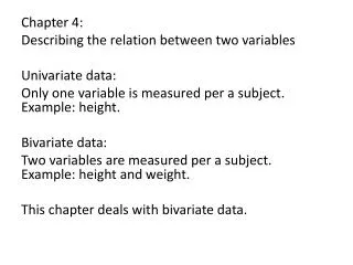
Bivariate data is data in which two variables are measured on an individual. The response variable is the variable whose value can be explained or determined based upon the value of the predictor variable. A lurking variable is one that is related to the response and/or predictor variable, but is excluded from the analysis
A scatter diagram shows the relationship between two quantitative variables measured on the same individual. Each individual in the data set is represented by a point in the scatter diagram. The predictor variable is plotted on the horizontal axis and the response variable is plotted on the vertical axis. Do not connect the points when drawing a scatter diagram.
EXAMPLE Drawing a Scatter Diagram The following data are based on a study for drilling rock. The researchers wanted to determine whether the time it takes to dry drill a distance of 5 feet in rock increases with the depth at which the drilling begins. So, depth at which drilling begins is the predictor variable, x, and time (in minutes) to drill five feet is the response variable, y. Draw a scatter diagram of the data. Source: Penner, R., and Watts, D.G. “Mining Information.” The American Statistician, Vol. 45, No. 1, Feb. 1991, p. 6.
Two variables that are linearly related are said to be positively associated when above average values of one variable are associated with above average values of the corresponding variable. That is, two variables are positively associated when the values of the predictor variable increase, the values of the response variable also increase.
Two variables that are linearly related are said to be negatively associated when above average values of one variable are associated with below average values of the corresponding variable. That is, two variables are negatively associated when the values of the predictor variable increase, the values of the response variable decrease
The linear correlation coefficient or Pearson product moment correlation coefficient is a measure of the strength of linear relation between two quantitative variables. We use the Greek letter (rho) to represent the population correlation coefficient and r to represent the sample correlation coefficient. We shall only present the formula for the sample correlation coefficient.
Properties of the Linear Correlation Coefficient 1. The linear correlation coefficient is always between -1 and 1, inclusive. That is, -1 <r< 1. 2. If r = +1, there is a perfect positive linear relation between the two variables. 3. If r = -1, there is a perfect negative linear relation between the two variables. 4. The closer r is to +1, the stronger the evidence of positive association between the two variables. 5. The closer r is to -1, the stronger the evidence of negative association between the two variables.
Properties of the Linear Correlation Coefficient 6. If r is close to 0, there is evidence of no linear relation between the two variables. Because the linear correlation coefficient is a measure of strength of linear relation, r close to 0 does not imply no relation, just no linear relation. 7. It is a unitless measure of association. So, the unit of measure for x and y plays no role in the interpretation of r.
EXAMPLE Drawing a Scatter Diagram and Computing the Correlation Coefficient • For the following data • Draw a scatter diagram and comment on the type of relation that appears to exist between x and y. • (b) By hand, compute the linear correlation coefficient.
EXAMPLE Determining the Linear Correlation Coefficient Determine the linear correlation coefficient of the drilling data.
A linear correlation coefficient that implies a strong positive or negative association that is computed using observational data does not imply causation among the variables.
Chapter 4Describing the Relation Between Two Variables 4.2 Least-squares Regression
EXAMPLE Finding an Equation that Describes a Linear Relation Using the following sample data: (a) Find a linear equation that relates x (the predictor variable) and y (the response variable) by selecting two points and finding the equation of the line containing the points. (b) Graph the equation on the scatter diagram. (c)Use the equation to predict y if x = 5.
The difference between the observed value of y and the predicted value of y is the error or residual. That is residual = observed - predicted Compute the residual for the prediction corresponding to x = 5.
EXAMPLE Finding the Least-squares Regression Line Using the sample data: (a) Find the least-squares regression line. (b) Interpret the slope and intercept. (c) Predict y if x = 5. (d) Compute the residual for x = 5. (e) Draw the least-squares regression line on the scatter diagram of the data.
EXAMPLE Computing the Sum of Squared Residuals Compute the sum of squared residuals for the line describing the relation between x and y that was obtained using two points. Compute the sum of squared residuals for the least-squares regression line. Which is smaller?
EXAMPLE Finding the Least-squares Regression Line • Find the least-squares regression line for the drilling data. • Use the line to predict the drilling time at x = 130 feet. • Should the line be used to predict the drilling time at x = 400 feet? Why? • Interpret the slope and y-intercept.