Galactic Supernova Detection Strategies: Virgo-LAL Group Comparison
250 likes | 352 Views
This study compares burst search methods for detecting the next Galactic supernova, focusing on amplitudes and network strategies. The analysis includes burst search methods, coincidences, coherent methods, and event confirmation through comparison of filtering algorithms. Efficiencies and strategies for different network configurations are examined.

Galactic Supernova Detection Strategies: Virgo-LAL Group Comparison
E N D
Presentation Transcript
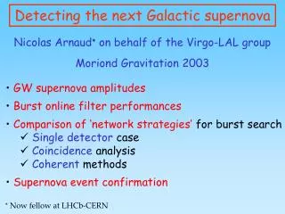
Detecting the next Galactic supernova Nicolas Arnaud on behalf of the Virgo-LAL group Moriond Gravitation 2003 • GW supernova amplitudes • Burst online filter performances • Comparison of ‘network strategies’ for burst search • Single detector case • Coincidence analysis • Coherent methods • Supernova event confirmation Now fellow at LHCb-CERN
Virgo cluster Comparison of maximum GW amplitudes 10 5 SNR=1 Milky Way Onecan hardly hope detecting a supernova outside Milky Way
See gr-qc/0210098 Burst search methods • Large variety of waveforms simulated numerically • Robust filters needed • Fast (and simple) filters required for online analysis • Benchmark developped @ LAL to study the performances • of the different filtering algorithms: • Zwerger-Müller simulated waveform catalog • averaged (realistic !?!) detection distance estimations • Test false alarm sensitivity to the data whitening • limits on remaining line amplitudes after whitening • ROC diagrams • detection efficiency versus false alarm rate • Timing resolution needed for coincidences between interferometers and other types of detectors (g, n, telescopes…)
Network data analysis strategies • Only way to properly separate real GW events from • transient noises located in a single interferometer • Two main sets of methods: • coincidence searches based on lists of selected events • provided by each interferometer • coherent searches • Data flows merged together while being analyzed • The latter approach is expected to be more efficient as • it includes all possible signal contributions while the • former uses ‘binary’ diagnostics – signal present/absent • Model of network detection quantitative comparison • between these two possibilities through ROC diagrams Detection efficiency vs false alarm rate per bin
IFO Beam pattern functions IFO Angular response Comparing Virgo-LIGO IFOs Declination d Right ascension a • Same components • Min/Max locations differ • 2 maxima ( detector) • 4 minima (blind detector)
Network Model: • Gaussian burst • width = 1 ms • ‘typical’ burst • Identical IFOs • ‘optimal situation’ • focus on the geographical • quality of the network • IFOs cannot move! • IFO Beam Patterns • Time delays between IFOs • Wiener filtering • Timing accuracy: Single detector ROC 50% efficiency 10 For SNRopt = 10, a 50% detection efficiency requires a false alarm rate of ~ 1 / second ! No hope to detect such burst in a single IFO with high confidence level
Coincidences: simulation procedure • Lists of events first computed in each IFO of the network • As consecutive filter outputs are strongly correlated, one • clusters data exceeding the threshold: • Event = (SNR, time, IFO name) with SNR and time • corresponding to the maximum filter output • in a set of consecutive data above the threshold • Clusterisation • [only important at high (single detector) false alarm rate] • Events (ri,ti, IFOi) and (rk, tk, IFOk) are compatibleif • | ti – tk | dist( IFOi, IFOk) + htiming (Si2 + Sk2) • A multiple coincidence between IFOs occurs when all • pairs of detectors are compatible • Focus on optimal SNR = 10 (expected @ Galactic center) Choosen equal to 1
Twofold coincidences 3 IFO network: Virgo + the 2 LIGO detectors Optimal SNR = 10 • Clearly better results for the • two LIGO-configuration: • Close detectors less random coincidences allowed between them • ‘Parallel’ orientations better pattern correlation with GW signals • Slower efficiency decrease • with increasing false alarm rate • w.r.t. the single detector case 60% efficiency
Coincidences in Virgo-LIGO network • Best strategy: • twofold coincidences • (at least 2 among 3) • Single detector less efficient • than coincidences • Threefold coincidences • too seldom • At very small false alarm rate, • the two LIGO detectors are • almost independent from Virgo 50% efficiency 30% Larger networks more promising / suitable
Full network coincidences 6 IFOs Network Requiring from 2 to 6 detections in the network • Twofold coincidences quite • likely even at small false • alarm rate • Threefold coincidences • also possible • Larger coincidences much more • seldom difficult to tighten • the compatibility test by • requiring in addition that the • coincidence defines well a • possible source location • in the sky 60% efficiency 40% efficiency
Coherent analysis • Coherent statistics derivated from the network likelihood • ratio (product of the single detector likelihood ratios) • [accurate for Gaussian and independent noises] • Adapted to burst case from pioneering works • Pai et al. PRD 64 (2001) Newtonian binary inspirals • Finn, PRD 63 (2001) comparison coincident/coherent • approaches in a simplified 2 detector network model • More efficient than coincidence methods • Benefits from all detector outputs without a priori • on the absence/presence of signals in the various IFOs • Requires an additional hypothesis: a source location • in the sky to shift and merge properly the IFO data • Covering the whole sky requires a set of coherent • filters (~ few thousands) running in parallel while • a single coincidence procedure is enough
Coherent ROC diagram in Virgo-LIGO ROC computed assuming known the source location SNRopt = 10 • Significant improvement • in detection efficiency • with respect to the • coincidence case • Efficiency remains above • 60% for SNRopt = 10 even • at a false alarm rate of • 1 per week! • Still no real hope to detect • a weak signal (SNRopt 5) • in the 3 interferometer • Virgo-LIGO network
Full network coherent ROC SNRopt = 10 ROC computed assuming known the source location • Clear enhancement of • detection efficiencies • by going from three to • six detectors • Almost certain detection • for SNRopt = 10 • Still more than 80% • efficiency @ SNRopt = 7.5 • Efficiency remains limited • @ SNRopt = 5 and below Coherence methods appear promising for linear filters
Comparing coincident/coherent analysis Even after false alarm rescaling, coherent methods show better detection efficiencies than coincidence analysis. Difference greater if one ‘simply’ wants to confirm a supernova signal triggered by other types of detectors: source position known can choose the right coherent filter! 1% / second @ 20 kHz Confirmations likely even in coincidence analysis Ex:False alarm suitable for burst confirmation:5 10-7 / bin Confirmation efficiencies for SNRopt = 10
Outlook • Detecting the next Galactic supernova remains challenging! • The larger the network, the better the detection efficiency • [Obvious but improvements from 3 to 6 IFOs are really significant] • Coincidence analysis seem not have detection efficiencies • high enough @ small false alarm rates • Coherent analysis more promising / more difficult to use • more computationally expensive • require complete data exchanges • cannot work for non-linear filters • More in-depth simulations needed but limiting analysis • to coincidences is clearly not optimal • Confirming a Galactic SN is more likely in both approaches • One just needs to be ready for the next one…
log. scale Supernova rate SN distribution uniform only beyond the Virgo cluster Virgo cluster Bump • SN rate data taken • from Cappellaro et al. • A&A 351, 459 (1999) • Mean rate: • (0.680.20) Snu • Tully catalog of galaxies • (2367 up to 40 Mpc) • used to compute the • rate vs. distance curves • cdsweb.u-strasbg.fr/cgi-bin/Cat?VII145 • Galactic Rate: • from 1/20 to 1/40 years-1 • Better not to miss • the ‘next’ one… 1 / year
Simulated waveform amplitudes hmax 1/distance Comparison of maximum GW amplitudes • SNR isocurves: • box GW signal @ hmax • width = 1 ms • white noise of RMS • 4 10-21 (Virgo min) • averaged pattern • «suboptimal filtering» Virgo cluster Apart for 1 optimistic simulation, one can hardly hope detecting a supernova outside Milky Way 10 5 1 Zwerger Müller (ZM) signals (A&A 320 1997): dmean = 27.5 1.1 kpc with threshold ~ 5 and optimal pattern Milky Way
Spatial and angular distributions Thin disk Galactic model: Cylindrical coordinates Source distribution probability with d = 3.5 kpc and H = 325 pc Celestial Coordinates (a, sind) • Non uniform angular distrib. • for a given sidereal time • But:Earth proper motion • averages this diagram • detection efficiencies at • given SNR are very close • to the uniform angular • distribution case • SNR depends on distance • @ dmean ~ 11 kpc, can expect • an optimalSNRopt ~ 10 (ZM) Likely visible SN Tails hardly visible
Burst search performances: ROC • NF:energy Filter • [ similar to Excess • Power Statistics ] • MF: mean Filter • [ averaging data ] • SF, OF, ALF: • Filters based on a • linear fit of data • Slope Filter • Offset Filter • ALF [quadratic • sum of SF and OF • once decorrelated] • Filters • not matched • with signal • real situation SNR = 5 signal: no angular pattern taken into account SF ALF shows the best results OF NF ALF MF 1 alarm/hour Normalized (/ bin)
Burst search performances:timing accuracy • Promising results for Gaussian bursts (width w): • Systematical bias computed trough MC simulations • Statistical errors smaller than w for SNR large enough • Situation less good for realistic (‘ZM-like’) bursts • Difficult to define a correct arrival time for a signal • full of peaks with similar magnitudes • timing precision both depends on the particular • signal and on the filter used to search it! stiming w for the best filters
Simulation main characteristics • Interferometers located at their real positions on Earth • Virgo, LIGO Hanford and Livingston (4 km), GEO, TAMA • ACIGA (orientation optimized w.r.t. the other detectors) • Focus on the ‘geographical complementarity’ between IFOs: • identical detectors • best network potential [future sensitivities unknown] • Emphasis on three particular configurations: • The two LIGO detectors (almost parallel) • Virgo + LIGO • The full set of six interferometers • Sources uniformly distributed in the sky • Signal amplitude defined by the maximal S/N SNRopt • Beam pattern functions and timing delays generated • Gaussian GW burst of millisecond width, • searched with matched filtering [‘generic’ burst] Mean matched filter output assuming an optimal IFO orientation
Gaussian burst width = 1 ms ! + IFO Beam Patterns + Wiener filtering Single detector ROC 1 ms 50% efficiency Timing error RMS S (w = 1 ms) Filter output ~ 5 For SNRopt = 10, a 50% detection efficiency requires a false alarm rate of ~ 1 / second ! No hope to detect such burst in a single IFO with high confidence level Fit S = 1.45 / (filter output) valid for outputs 5-6
Coincidence strategy comparison • The larger the network, • the better the detection • efficiency at a given • false alarm rate • A three IFO-network • seems not efficient enough • Key point: number of • IFO in the network • rather than their • particular locations • [All IFOs have roughtly • identical contributions • in the full network] 60% 30%
Coherent analysis and false alarm rates • The false alarm rate of a single coherent filter needs to be rescaled • as many such templates must be used in parallel to cover the whole sky • Error in source direction • errors in the relative time shifts • applied to the different IFO outputs • Can compute a metric describing this loss as a function of the • direction mismatch in the two coordinates (a, X=sind) • Can apply the Owen formalism to this 2D parameter space to • estimate the number of templatesN needed to cover it • For a 97% minimal match, one gets N ~ 5000 both for the Virgo-LIGO • network and for the full network of six IFOs. • Template correlation ? • Unknown but certainly non zero as templates are close • Scaling by a factor 1000 the coherent false alarm rates seems • accurate (and possibly conservative) Assumed to be the main sources of loss in the coherent statistics [Pai et al.]