Download
1 / 36
360 likes | 472 Views
This document outlines best practices for model calibration and evaluation, emphasizing systematic approaches to enhance model fit, predictiveness, and parameter estimates. It includes guidelines for using both deterministic and statistical methods to quantify prediction uncertainty. Key practices involve utilizing a wide range of observation data, carefully assigning weights to account for observation error, and considering alternative models to improve accuracy. Additionally, strategies for modeling predictions, such as regression analysis and confidence interval calculations, are discussed to ensure reliable and interpretable results.

E N D
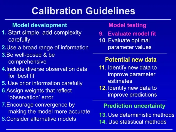
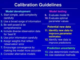
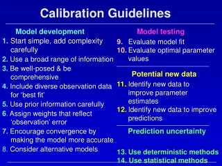
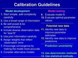
Calibration Guidelines Model development Model testing 9.Evaluate model fit 10.Evaluate optimal parameter values 11. Identify new data to improve parameter estimates 12. Identify new data to improve predictions 13.Use deterministic methods 14.Use statistical methods 1.Start simple, add complexity carefully 2. Use a broad range of information 3. Be well-posed & be comprehensive 4. Include diverse observation data for ‘best fit’ 5.Use prior information carefully 6. Assign weights that reflect ‘observation’ error 7. Encourage convergence by making the model more accurate 8. Consider alternative models Potential new data Prediction uncertainty
Guideline 13:Evaluate Prediction Uncertainty and Accuracy Using Deterministic Methods • Use regression to evaluate predictions • Consider model calibration and Post-Audits from the perspective of the predictions. • Book Chapter 14
Using regression to evaluate predictions • Determine what model parameter values or conditions are required to produce a prediction value, such as a concentration value exceeding a water quality standard. • How? Modify the model to simulate the prediction conditions (e.g. longer simulation time, add pumping, etc.). Include the prediction value as an ‘observation’ in the regression; use a large weight. • If the model is thought to be a realistic representation of the true system: • If estimated parameter values are reasonable, and the new parameter values do not produce a bad fit to the observations: • The prediction value is consistent with the calibrated model and observation data. The prediction value is more likely to occur under the simulated circumstances. • If the model cannot fit the prediction, or a good fit requires unreasonable parameter values or a poor fit to the observations: • The prediction value is contradicted by the calibrated model and observation data. The prediction value is less likely to occur under the simulated circumstances.
Using regression to evaluate predictions • This method does not provide a quantifiable measure of prediction uncertainty, but it can be useful to understand the dynamics behind the prediction of concern.
Guideline 14: Quantify Prediction Uncertainty Using Statistical Methods Goal: Present predicted values with uncertainty measured; often intervalsTwo Categories of Statistical Methods: 1. Inferential Methods - Confidence Intervals 2. Sampling Methods- Deterministic with assigned probability - Monte Carlo (random sampling)
Guideline 14:Quantify Prediction Uncertainty Using Statistical Methods • Advantage of using regression to calibrate models: use related inferential methods to quantify some prediction uncertainty. • Sources of uncertainty accounted for: • Error and scarcity of observations and prior information • Lack of model fit to observations and prior information • Translated through uncertainty in the parameter values • More system aspects defined with parameters more realistic uncertainty measures • Intervals calculated using inferential statistics do not easily include uncertainty in model attributes not represented with parameters, and nonlinearity can be a problem even for nonlinear confidence intervals. Both can be addressed with sampling methods.
Confidence Intervals • Confidence intervals are ranges in which the true predictive quantity is likely to occur with a specified probability (usually we use 95%, which means the significance level is 5%). • Linear confidence intervals on parameter values calculated as • bj 2sbjwhere sbj = s2(XTwX)–1jj • Linear confidence intervals on parameter values reflect • Model fit to observed values (s2) • Observation sensitivities (X; xij = y’i/ bj) • Accuracy of the observations as reflected in the weighting (w) • Linear confidence intervals on predictions: propagate para-meter uncertainty and correlation using prediction sensitivities • zk cszkwhere szk = (zk/b) [s2(XTwX)–1] (zk/b)
Types of confidence intervals on predictions • Individual • If only one prediction is of concern. • Scheffe simultaneous • If the intervals for many predictions are constructed and you want intervals within which all predictions will fall with 95% probability • Linear: Calculate interval as zk cszk • For individual intervals, c2. • For Scheffe simultaneous c>2 • Nonlinear: • Construct a nonlinear 95% confidence region on the parameters and search the region boundary for the parameter values that produce the largest and smallest value of the prediction. Requires a regression for each limit of each confidence interval.
Objective function surface for the Theis equation example (Book, fig. 5-3) • Choosing a significance level identifies a confidence region defined by a contour. • Search the region boundary (the contour) for parameter values that produce the largest and smallest value of the prediction. These form the nonlinear confidence interval. • The search requires a nonlinear regression for each confidence interval limit. • Nonlinear intervals are always Sheffe intervals
Book fig 8.3, p. 179. Modified from Christensen and Cooley, 1999
Example: Confidence Intervals on Predicted Advective-Transport Path Plan View Book fig 2.1a, p. 22 Linear individual intervals Book fig 8.15a, p. 210
Linear Individual Linear Simultaneous (Scheffe d=NP) Book fig 8.15, p. 210 Nonlinear Simultaneous (Scheffe d=NP) Nonlinear Individual
The limits of nonlinear intervals are always a model solution Confidence intervals on advective-transport predictions at 10, 50, and 100 years. (Hill and Tiedeman, 2007, p. 210) Nonlinear individual intervals Linear individual intervals
Suggested strategies when using confidence and prediction intervals to indicate uncertainty • Calculated intervals do not reflect model structure error. Generally indicate the minimum likely uncertainty (though nonlinearity makes this confusing). • Include all defined parameters. If available, use prior information on insensitive parameters so that the intervals are not unrealistically large. • Start with linear confidence intervals, which can be calculated easily. • Test model linearity to determine the likely accuracy of linear intervals. • If needed and as possible, calculate nonlinear intervals (in PEST-2000 as the Prediction Analyzer; in MODFLOW-2000 as the UNC Package; working on UCODE_2005). • Use simultaneous intervals if multiple values are considered or the value is not completely specified before simulation. • Use prediction intervals (versus confidence intervals) to compare measured and simulated values. (not discussed here)
Use deterministic sampling with assigned probabilityto quantify prediction uncertainty • Samples are generated using deterministic arguments like different interpretations of the hydrogeologic framework, recharge distribution, and so on. • Probabilities are assigned based on the support the different options have from the available data and analyses.
Use Monte Carlo methods to quantify prediction uncertainty • Used to estimate prediction uncertainty by running forward model many times with different input values. • The different input values are selected from a statistical distribution. • Fairly straightforward to describe results and to conceptualize process. • Can generate parameter values using measures of parameter uncertainty and correlation calculated from regression output. Results are closely related to confidence intervals. • Can also use sequential, indicator, other ‘simulation’ methods to generate realizations with specified statistical properties. • Need to be careful in generating parameter values / realizations. The uncertainty of the prediction can be greatly exaggerated by using realizations that clearly contradict what is known about the system. • Good check – only consider generated sets that respect known hydrogeology and produce a reasonably good fit to any available observations.
Example of using Monte Carlo methods to quantify prediction uncertainty Example from Poeter and McKenna (GW, 1995) • Synthetic aquifer with proposed water supply well near a stream. • Could the proposed well be contaminated from a nearby landfill? • Used Monte Carlo analysis to evaluate the uncertainty of the predicted concentration at the proposed supply well. Book p. 343
Monte Carlo approach from Poeter and McKenna 1995 • Generate 400 realizations of the hydrogeology using indicator kriging. • Generate using the statistics of hydrofacies distrubutions. Assign K by hydrofacies type. • Generate using also soft data about the distribution of hydrofacies. Assign K by hydrofacies type. • Generate using also soft data about the distribution of hydrofacies. Assign K by regression using head and flow observations. • For each realization simulate transport using MT3D. Save predicted concentration at the proposed well for each run. • Construct histogram of the predicted concentrations at the well. True concentration Book p. 343
Use inverse modeling to produce more realistic prediction uncertainty • The 400 models were each calibrated to estimate the optimal K’s for the hydrofacies. • Realizations were eliminated if: • Relative K values not as expected • K’s unreasonable • Poor fit to the data • Flow model did not converge • Remaining realization: 2.5% = 10 • Simulate transport using MT3D. • Construct histogram. • Huge decrease in prediction uncertainty – prediction much more precise than with other types of data • Interval includes the true concentration value – the greater precision appears to be realistic True concentration
Software to Support Analysis of Alternative models • MMA: Multi-Model Analysis Computer Program • Poeter, Hill, 2007. USGS. • Journal article: Poeter and Anderson, 2005, GW • Evaluate results from alternative models of a single system using the same set of observations for all models. • Can be used to • rank and weight models, • calculate model-averaged parameter estimates and predictions, and • quantify the uncertainty of parameter estimates and predictions in a way that integrates the uncertainty that results from the alternative models. • Commonly the models are calibrated by nonlinear regression, but could be calibrated using other methods. Use MMA to evaluate calibrated models.
MMA (Multi-Model Analysis) • By default, models are ranked using • Akaike criteria AIC and AICc (Burnham and Anderson, 2002) • Bayesian methods BIC and KIC (Neuman, Ming, and Meyer).
MMA: How do the default methods compare? • Burnham and Anderson (2002) suggest that use of AICc is advantageous because • AICc does not assume that the true model is among the models considered. • So, AICc tends to rank more complicated models (models with more parameters) higher as more observations become available. This does make sense, but…. What does it mean?
Model discrimination criteria n= NOBS + NPR AIC = n ln(sML2) + 2 NP 2 NP (NP+1) (n – NP – 1) AICc= n ln(sML2) + 2 NP+ BIC = n ln(sML2) + NP ln(n) sML2 = SSWR/n = the maximum-likelihood estimate of the variance. First term tends to decrease as parameters are added Other terms increase as parameters are added (NP inc.) More complicated models are preferred only if the decrease of the first term is greater than the increase of the other terms.
Plot the added terms to see how • much the first term has to • decrease for a more complicated • model to be preferable. • Plots a and b show that as NOBS • increases • AICc AIC. • AICc gets smaller, so it is easier for models with more parameters to compete. • BIC increases! It becomes harder for models with more parameters to compete. • Plot a and c show that when • NOBS and NP both increase • AIC and AICc increase proportionately. • BIC increases more. 30 30 30
KIC KIC = (n-NP) ln(sML2) – NP ln(2p) +ln|XTwX| Couldn’t evaluate for the graph because the last term is model dependent. Asymptotically, performs like BIC.
MMA: Default method for calculating posterior model probabilities • Use criteria differences, “delta values”. For AICc, • Posterior model probability=Model weights=Akaike Wts: • Inverted evidence ratio, as a percent = 100 pj/plargest = the evidence supporting model i relative to the best model, as a percent. So if 5%, the data provide 5% as much support for that model as for the most likely model pi
Example(MMA documentation) • Problem: Remember that Delta= • The delta value is the difference, regardless of how large the criterion is. The values can become quite large if the number of observations is large. • This can produce some situations that don’t make much sense. • A tiny percent difference in the SSWR can result in one model being very probable and the other not at all probable. • Needs more consideration.
MMA: Other Model criteria and weights • Very general. • MMA includes an equation interface contributed to the JUPITER API by John Doherty. • Also, values from a set of models such as the largest, smallest, or average prediction can be used.
MMA: Other features • Can omit models with unreasonable estimated parameter values. These are through user-defined equation like Ksand<Kclay. • Always omits models for which regression did not converge. • Requires specific files to be produced for each model being analyzed. These are produced by UCODE_2005, but could be produced by other models. • Input structure uses JUPITER API input blocks, like UCODE_2005
BEGIN MODEL_PATHS TABLE nrow=18 ncol=1 columnlabels PathAndRoot ..\DATA\5\Z2\1\Z ..\DATA\5\Z2\2\Z ..\DATA\5\Z2\3\Z ..\DATA\5\Z2\4\Z ..\DATA\5\Z2\5\Z ..\DATA\5\Z3\1\Z ..\DATA\5\Z3\2\Z ..\DATA\5\Z3\3\Z ..\DATA\5\Z3\4\Z ..\DATA\5\Z3\5\Z ..\DATA\5\Z4\1\Z ..\DATA\5\Z4\2\Z ..\DATA\5\Z4\3\Z ..\DATA\5\Z4\4\Z ..\DATA\5\Z4\5\Z ..\DATA\5\Z5\1\Z ..\DATA\5\Z5\2\Z ..\DATA\5\Z5\3\Z END MODEL_PATHS Example complete input file for simplest situation
MMA: Uncertainty Results Head, in meters
Exercise • Considering the linear and nonlinear confidence intervals on slide 11 of this file, answer the following questions • Why are the linear simultaneous Scheffe intervals larger than the linear individual intervals? • Why are the nonlinear intervals so different?
Important issues when considering predictions • Model predictions inherit all the simplifications and approximations made when developing and calibrating the model!!! • When using predictions and prediction uncertainty measures to help guide additional data collection and model development, do so in conjunction with other site information and other site objectives. • When calculating prediction uncertainty include the uncertainty of all model parameters, even those not estimated by regression. This helps the intervals reflect realistic uncertainty.
Calibration Guidelines Model development Model testing 9.Evaluate model fit 10.Evaluate optimal parameter values 11. Identify new data to improve parameter estimates 12. Identify new data to improve predictions 13.Use deterministic methods 14.Use statistical methods 1.Start simple, add complexity carefully 2. Use a broad range of information 3. Be well-posed & be comprehensive 4. Include diverse observation data for ‘best fit’ 5.Use prior information carefully 6. Assign weights that reflect ‘observation’ error 7. Encourage convergence by making the model more accurate 8. Consider alternative models Potential new data Prediction uncertainty
Warning! • Most statistics have limitations. Be aware! • For the statistics used in the Methods and Guidelines, validity depends on accuracy of model, and model being linearwith respect to the parameters • Evaluate likely model accuracy using • Model fit (Guideline 8) • Plausibility of optimized parameter values (Guideline 9) • Knowledge of simplifications and approximations • Model is nonlinear, but these methods were found to be useful. Methods not useful if the model is too nonlinear.
The 14 Guidelines • Organized common sense with new perspectives and statistics • Oriented toward clearly stating and testing all assumptions • Emphasize graphical displays that are • statistically valid • informativeto decision makers We can do more with our data and models!! mchill@usgs.gov tiedeman@usgs.gov water.usgs.gov