Very Basic Statistics
Very Basic Statistics. Course Content. Data Types Descriptive Statistics Data Displays. Data Types. Variables. Quantitative Variable A variable that is counted or measured on a numerical scale Can be continuous or discrete (always a whole number). Qualitative Variable

Very Basic Statistics
E N D
Presentation Transcript
Course Content • Data Types • Descriptive Statistics • Data Displays
Variables • Quantitative Variable • A variable that is counted or measured on a numerical scale • Can be continuous or discrete (always a whole number). • Qualitative Variable • A non-numerical variable that can be classified into categories, but can’t be measured on a numerical scale. • Can be nominal or ordinal
Continuous Data • Continuous data is measured on a scale. • The data can have almost any numeric value and can be recorded at many different points. • For example • Temperature (39.25oC) • Time (2.468 seconds) • Height (1.25m) • Weight (66.34kg)
Discrete Data • Discrete data is based on counts, for example; • The number of cars parked in a car park • The number of patients seen by a dentist each day. • Only a finite number of values are possible e.g. a dentist could see 10, 11, 12 people but not 12.3 people
Nominal Data • A Nominal scale is the most basic level of measurement. The variable is divided into categories and objects are ‘measured’ by assigning them to a category. • For example, • Colours of objects (red, yellow, blue, green) • Types of transport (plane, car, boat) • There is no order of magnitude to the categories i.e. blue is no more or less of a colour than red.
Ordinal Data • Ordinal data is categorical data, where the categories can be placed in a logical order of ascendance e.g.; • 1 – 5 scoring scale, where 1 = poor and 5 = excellent • Strength of a curry (mild, medium, hot) • There is some measure of magnitude, a score of ‘5 – excellent’ is better than a score of ‘4 – good’. • But this says nothing about the degree of difference between the categories i.e. we cannot assume a customer who thinks a service is excellent is twice as happy as one who thinks the same service is good.
Task 1 • Look at the following variables and decide if they are qualitative or quantitative, ordinal, nominal, discrete or continuous • Age • Year of birth • Sex • Height • Number of staff in a department • Time taken to get to work • Preferred strength of coffee • Company size
Session Content • Measures of Location • Measures of Dispersion
Common Measures • Measures of location summarise the data with a single number • There are three common measures of location • Mean • Mode • Median • Quartiles are another measure
Mean • The mean (more precisely, the arithmetic mean) is commonly called the average • In formulas the mean is usually represented by read as ‘x-bar’. • The formula for calculating the mean from ‘n’ individual data-points is; X bar equals the sum of the data divided by the number of data-points
Advantages basic calculation is easily understood all data values are used in the calculation used in many statistical procedures. Disadvantages It may not be an actual ‘meaningful’ value, e.g. an average of 2.4 children per family. Can be greatly affected by extreme values in a dataset. e.g. seven students take a test and receive the following scores. 40 42 45 50 53 54 99 The average score is 54.7 – but is this really representative of the group? If the extreme value of 99 is dropped, the average falls to 47.3 Pro’s & Con’s
Mode • The mode represents the most commonly occurring value within a dataset. • We usually find the mode by creating a frequency distribution in which we tally how often each value occurs. • If we find that every value occurs only once, the distribution has no mode. • If we find that two or more values are tied as the most common, the distribution has more than one mode.
Advantages easy to understand not affected by outliers (extreme values) can also be obtained for qualitative data e.g. when looking at the frequency of colours of cars we may find that silver occurs most often Disadvantages not all sets of data have a modal value some sets of data have more than one modal value multiple modal values are often difficult to interpret Pro’s & Con’s
Task 2 • The following values are the ages of students in their first year of a course 18, 19, 18, 25, 22, 20, 21, 45, 33, 20, 18, 18 • Find the mean age of the students • Find the modal value • In your opinion which is the better measure of location for this data set?
Median • Median means middle, and the median is the middle of a set of data that has been put into rank order. • Specifically, it is the value that divides a set of data into two halves, with one half of the observations being larger than the median value, and one half smaller. Half the data < 29 Half the data > 29 18 24 29 30 32
Finding the Median from Individual Data • Step 1:- Arrange the observations in increasing order i.e. rank order. The median will be the number that corresponds to the middle rank. • Step 2:- Find the middle rank with the following formula: Middle rank = ½*(n+1) • Step 3 – Identify the value of the median • If ‘n’ is an odd number the middle rank will fall on an observation. The median is then the value of that observation.
40 42 45 50 53 54 70 99 Position of Median = ½*(n+1) = 4.5 Median = Median = Finding the Median from Individual Data • If ‘n’ is an even number, the middle rank will fall between two observations. In this case the median is equal to the arithmetic mean of the values of the two observations
Advantages the concept is easy to understand the median can be determined for any type of data (with the exception of nominal) the median is not unduly influenced by extreme values in the dataset Disadvantages data must be arranged in rank order (ascending or descending) cannot combine medians in statistical calculations as with mean values Pro’s & Con’s
Task 3 • Using the student age data below, find the median age 18, 19, 18, 25, 22, 20, 21, 45, 33, 20, 18, 18
Quartiles • Also known as percentiles • Lower quartile - 25% of the data is below this • Position of Q1 = ¼*(n+1) • Upper quartile – 75% of the data is below this • Position of Q3 = ¾*(n+1) • If a quartile falls on an observation, the value of the quartile is the value of that observation. • For example, if the position of a quartile is 20, its value is the value of the 20th observation.
40 42 45 50 53 54 70 99 Position of Upper Quartile = ¾*(n+1) = 6.75 Upper quartile = data-point 6 + 0.75*(data-point 7 – data-point 6) Upper quartile = 54 + 0.75*(70 – 54) = 66 Quartiles • If a quartile lies between observations, the value of the quartile is the value of the lower observation plus the specified fraction of the difference between the two observations.
Task 4 • Using the student age data below find the upper and lower quartiles 18, 19, 18, 25, 22, 20, 21, 45, 33, 20, 18, 18
2 4 6 8 10 12 14 16 2 4 6 8 10 12 Report turnaround time (days) Common Measures • The dispersion in a set of data is the variation among the set of data values. • It measures whether they are all close together, or more scattered. Report turnaround time (days)
Common Measures • The four common measures of spread are • the range • the inter-quartile range • the variance • the standard deviation
Days 4 16 Range Range • The range is the difference between the largest and the smallest values in the dataset i.e. the maximum difference between data-points in the list. • It is sensitive to only the most extreme values in the list. The range of a list is 0 if and only if all the data-points in the list are equal.
Advantages best for symmetric data with no outliers easy to compute and understand good option for ordinal data Disadvantages doesn’t use all of the data, only the extremes very much affected if the extremes are outliers only shows maximum spread, does not show shape Pro’s & Con’s
Task 5 • Using the student age data find the range of the data. 18, 19, 18, 25, 22, 20, 21, 45, 33, 20, 18, 18
Inter-quartile Range • (upper quartile – lower quartile) • Essentially describes how much the middle 50% of your dataset varies • example: if all patients in a dentist surgery took more-or-less the same time to be treated with only one or two exceptionally quick or long appointments you would expect the inter-quartile range to be very small • but if all appointments were either very quick or very long, with few in between then the inter-quartile range would be larger.
Advantages Good for ordinal data Ignores extreme values More stable than the range because it ignores outliers Disadvantages Harder to calculate and understand Doesn’t use all the information (ignores half of the data-points, not just the outliers) Tails almost always matter in data and these aren’t included Outliers can also sometimes matter and again these aren’t included. Pro’s & Con’s
Task 6 • Using the student age data find the inter-quartile range. 18, 19, 18, 25, 22, 20, 21, 45, 33, 20, 18, 18
Variance and Standard Deviation (s2, s2) =(population notation, sample notation) • The variance (s2, s2)and standard deviation (s, s)are measures of the deviation or dispersion of observations (x) around the mean (m) of a distribution • Variance is an ‘average’ squared deviation from the mean
Mean 1 SD 1 SD Mean 1 SD 1 SD 8 10 12 4 6 8 10 12 14 16 Variance and Standard Deviation • The standard deviation (SD) is the square root of the variance. • small SD = values cluster closely around the mean • large SD = values are scattered Days
Variance and Standard Deviation • The following formulae define these measures Population Sample
Variance • Advantages: • uses all of the data values • Disadvantages: • the variance is measured in the original units squared • extreme values or outliers effect the variance considerably • hard to calculate manually
Standard Deviation • Advantages: • same units of measurement as the values • useful in theoretical work and statistical methods and inference • Disadvantages: • hard to calculate manually
Task 7 • Using the student age data find the variance and the standard deviation 18, 19, 18, 25, 22, 20, 21, 45, 33, 20, 18, 18
Session Summary • Measures of Location • Mean • Mode • Median • Quartiles • Measures of Dispersion • Range • Interquartile Range • Variance • Standard Deviation
Session Content • Histograms • Run charts • Box plots • Bar charts • Pareto charts • Pie charts • Scatter plots • Contingency tables