Download

1 / 37
370 likes | 525 Views
MICROARRAYS D’EXPRESSIÓ ESTUDI DEL FACTOR DE TRANSCRIPCIÓ ASH2. M. Corominas : mcorominas@ub.edu. Spotted array experiment. 1. Prepare sample. 4. Print microarray. Test. Reference. 2. Label with fluorescent dyes. 5. Hybridize to microarray. 3. Combine cDNAs. 6. Scan.

E N D
MICROARRAYS D’EXPRESSIÓ ESTUDI DEL FACTOR DE TRANSCRIPCIÓ ASH2 M. Corominas: mcorominas@ub.edu
Spotted array experiment 1. Prepare sample. 4. Print microarray. Test Reference 2. Label with fluorescent dyes. 5. Hybridize to microarray. 3. Combine cDNAs. 6. Scan.
Spotted microarrays rely on delivery technologies to place biologic material (purified cDNA, oligonucleotides) onto allocated locations of the chip. (competitive hybridization: Cy3vsCy5)
Drosophilamelanogaster Wolpert (2001)
ash2 - member of atrithorax group Belongs to multiprotein chromatin remodeling complexes • Polycomb (PcG) :transcriptionalrepression • trithorax (trxG): transcripcional activation Transcriptional Regulator
Direct PCR from Bacterial Growth using vector-specific primers Analysis of PCR results by electrophoresis Spotting on slide TYPES OF MICROARRAYS 1)From full length cDNA Plates from the Berkeley Drosophila Gene Collection with 384 wells (clones) each: DGC1.0 and 2.0 Aprox. 12000 genes in total
TYPES OF MICROARRAYS 2)From 400 bp amplicons a) correspond to approximately 75% of genes predicted in release 3.1 (gene specific primers kindly donated by Incyte Genomics and Brian Oliver, NIH). b) based on a novel annotation of the fly genome. It contains 21376 gene- specific probes. Performed and available from Eurogentec. Carried out in collaboration (ZMBH, Univ. of Heidelberg; DKFZ, MPI Molecular Genetics Computational Molecular Biology, Germany)
3)From oligonucleotides a) INDAC project: International Drosophila Array Consortium www.indac.net 70 mer oligonucleotides designed towards the 3’ end of the genes (based on the 3.1 release) with specific algorithms and synthesized by Illumina. b) Qiagen/Operon oligo set 70 mer oligonucleotides representing 13,664 genes designed from release 3.1 already available in the Plataforma de Transcriptòmica Serveis Científico-Tècnics UB- PCB
- RNA samples: - total RNA - polyA+ RNA - T7 polymerase amplified RNA - labeling method (competitive hybridization): - direct - indirect - positive and negative controls MIAME describes the Minimum Information About a Microarray Experiment that is needed to enable the interpretation of the results of the experiment unambiguously and potentially to reproduce the experiment. http://www.mged.org/Workgroups/MIAME/miame.html
Direct PCR from Bacterial Growth Analysis of PCR results by electrophoresis Spotting on slide Production of cDNA chips 17 plates from the Berkeley Drosophila Gene Collection with 384 wells (clones) each. Aprox. 5000 genes in total
Trizol RNA Extraction & Poly A+ Purification mRNA mRNA Cy5 test sample Cy3 control sample Hybridize Slide Hybridization of Chips mutant flies (ash2) wild-type flies Two-Step Fluorescent Labelling
532 nm 635nm -Integrate Data -Filter Data -Adjust dye bias -Calculate Ratios -Adjust Data -Set Thresholds Scanning of Chips Scan Slide fluorescent intensities for each cDNA, spot or gene fluorescent intensities for each cDNA, spot or gene GenePix
“Bad” Spots Filtering • Is the process in which spots that don’t look right are • discarded according to different criteria GenePix discards data according to internal filters like: x % pixels > Median Background intensity Convert Data 3.33 to further filter data. Spots were flagged as OK if: medianFx > mBx +/- XSD • Spots must pass filtering for both channels
log(F635Median-B635) log(F532Median-B532) Distribution for Good spots at both wavelengths 120 100 80 60 Number in each class 40 20 0 5 9 13 17 5.8 6.6 7.4 8.2 9.8 10.6 11.4 12.2 13.8 14.6 15.4 16.2 17.8 log (F Median - B)
Adjusting Ratios • A Ratio measures how much sample cDNA over control • cDNA we have of a given gene. This is: • Ratio = Intensity sample / Intensity control • Different measures for the ratios: • Ratio of Medians • Ratio of Means • Regression Ratio • Log (base 2) the ratios : • Makes variation of intensities and ratios of intensitiesmore independent of absolute magnitude. • Gives a more realistic sense of variation.
Multiple Experiment Comparison Modify data the same way in all experiments: - bad spots filtering methods - ratio (eg. Ratio of Medians) • adjust ratios: • mean centering • Normalization • main class centering
We expect: • few genes upregulated • few genes downregulated • most genes unchanged (log2 Ratio = 0) • Therefore: • a Normal distribution • with mean (all log2 Ratio ) = 0 • Draw distribution of Ratios and check mean: • if really not N: filter bad spots better • try to Normalize (mean = 0; SD = 1) • discard experiment • if close to N: adjust mean (product or sum) • Normalize (0; 1)
Norm log Ratio of Medians Experiment 1 Experiment 3 Experiment 2 Experiment 4 7 6 5 4 % Genes in Class 3 2 1 0 4 -7 0.7 1.8 2.9 5.1 6.2 -1.5 -5.9 -4.8 -3.7 -2.6 -0.4 log Ratio of Medians Class Multiple Experiment Comparison
Set method to select up or downregulated genes - higly subjective method like fold-change (eg. two, three) - semi-statistical method like Mean ± xSD • statistical method like SAM: • missing values imputed using a K-nearest Neighbor • computes a statistic • set threshold for statistic (to call significant genes) • will give you a FDR • set fold-change threshold
Mean Corr. Coef 0.88 Filtering of Bad Spots 140 95 Results 5139 different genes with FBgn in total 4163 different genes with FBgn (SAM INPUT) SAM 2.5% FDR 1.75 Foldchange
If a gene is downregulated in the mutant (ash2I1): • Ratio = F sample / F control <1 • log2 Ratio <0, because log2 1=0 • ash2 is in activation pathway • If a gene remains unchanged in the mutant (ash2I1): • Ratio = F sample / F control = 1 • log2 Ratio = 0, because log2 1=0 • ash2 is not regulating this gene • If a gene is upregulated in the mutant (ash2I1): • Ratio = F sample / F control > 1 • log2 Ratio > 0, because log2 1=0 • ash2 is in repression pathway
Controls and Quality assesment - Sequencing of some clones from the Collection plates - RT-PCR of some genes in a semiquantitative way - in situ hybridization - Western Blot - inmunolocalization - Northern Blot - Clonal Analysis
ASH2 RT-PCR + = wt - = ash2
Classification according to GO (Gene Ontology) • Gene Ontology is a “controlled vocabulary that can be • applied to all eukaryotes “. Each gene product is classi- • fied in one or more categories. • Is distribution of missexpressed genes significantly • different from the one of our initial set of genes? • maybe ash2 acts predominantly upon a group • of genes of similar function or pathway
Operon D. melanogaster Array 16416 spots 14593 70mer probes representing 13664 genes and 17899 transcripts POSITIVE CONTROLS • 10 A. thaliana oligos (TIGR spikes) - each printed 4 times by pin = 640 spots • 12 D. melanogaster oligos - each printed 17 times = 204 spots NEGATIVE CONTROLS • 12 Randomly Generated Negative Controls – printed several times = 188 spots • 352 Empty spots • 449 Buffer spots (hybridized with aRNA ISOash2I1 vs ISO)
2 TIFF images (Cy3 & Cy5) GAL file (gene matrix) Input GenePix Pro 4.0 Image analysis ANALYSIS LAYOUT Output 1 GPR file for experiment Input TIGR Express Converter 1.4.1 Output 1 MEV file for experiment
1 MEV file for experiment (total=5) Input TIGR MIDAS • Each experiment analyzed independently • Background filter applied • Normalization applied: Lowess (LOC) for each experiment independently Input EXCEL & TIGR MEV • Spike-in, negative and positive control Check • MA Plots • Experiment Comparison (Scatter Plots) • Relevant Genes Finding
TIGR spike-in Mix We can use the spikes to assess quality of experiment and analysis On chip: 10 A. thaliana oligos spotted 64 times each (4 times by pin) To add to labeling reaction: In vitro synthesized RNA from each gene at different proportions and quantities: For Amplification experiments we use the spikes diluted 1:500
TIGR spikes MA plot from an experiment with total RNA Experimental procedure and analysis seems good (spikes fall where expected)
TIGR Spikes Operon Arrays Insets ISO ash2I1 vs ISO L3 total RNA aRNA from L3 total RNA • 2 ug amplified to 70ug in 4h • 20ug of labelled aRNA - 60ug indirectly labelled
Amplification Test: totalRNA vs aRNA log2ratios Correlation coef = 0.94
Biological Replicates REPLICATE 1 REPLICATE 2
Amplified TIGR spikes (diluted 1:100) together with probes Biological Replicates Microarray Insets REPLICATE 1 REPLICATE 2
Biological Replicates Replicate 1 vs Rplicate 2 log2ratios Correlation coef = 0.92