Download
1 / 42
430 likes | 558 Views
Practical Lineage Tracing in Data Warehouses. Paper by Y. Cui and J. Widom Appeared in ICDE 2000 Presented by Royi Ronen in Seminar in Databases (236826), Winter 2009. Introduction. A visit to a computing center of a restaurant. View Menu(item,cost,price). Database. product(name,cost)

E N D
Practical Lineage Tracing in Data Warehouses Paper by Y. Cui and J. Widom Appeared in ICDE 2000 Presented by Royi Ronen in Seminar in Databases (236826), Winter 2009
A visit to a computing center of a restaurant View Menu(item,cost,price) Database product(name,cost) labor(id,cost) overheads(name,cost) operations(name,cost) > What made the price high? How can we solve the problem?
The Lineage Problem • Given: • A view V • A database instance D • A data item d in a tuple in V(D) • Find: • All data items that produced d and the process in which d was produced אילן יוחסין, שושלת יוחסין Lineage =
Motivation • In many data analysis and management scenarios, the source of the data is valuable • OLAP (online analytical processing) • When sources are of different qualities (certainty, reliability, etc.) • Scientific databases • Top-down Datalog evaluation • On-line monitoring • This is the first research to discuss the problem
Example - I DBSchema View
Example - II Promising
Example - III • What is the exact set of data items which produced computer according to view Promising?
Tuple Lineage for one Operator • Let Op be an operator from {,,,} • Let T=Op(T1,…,Tm) , tT t’s lineage in (T1,…,Tm) according to Op is: Op-1<T1,…,Tm>= T*1,…,T*m where T*i are the maximal sets s.t. • (a) Op(T*1,…,T*m) = {t} • (b) T*i t*Ti : Op(T*1,…,{t*},…,T*m) lineage tuples derive exactly t every tuple contributes to t
Discussion • Op(T*1,…,T*m) = {t} Alone, this condition could be met even if many non-relevant tuples are in T*i • T*i t*Ti : Op(T*1,…,{t*},…,T*m) Alone, this condition could be met by many tuples not at all related to t • Together, the two conditions define the lineage
Example x,sum(Y)(T) T(X,Y) t= Lineage of (a,6)
Tuple lineage for a view • A view definition has many operators • We assume that views are evaluated as a query tree, bottom-up • Thelineage in D of a tuple t accordingto v(D), v-1D(t), is defined by recursively generalizing tuple lineage for an operator • Basis: t contributes to itself in V, when the view is just a table • Step: previous definition of an operator • Transitivity: if t1 contributes to t2, and t2 contributes to t3, then t1 contributes to t3
Example V = X,sum(Y) (Y>0(RS))
Segment 1 Segment 2 Canonical form for ASPJ views • Any aggregate-select-project-join (ASPJ) view can be transformed to an equivalent canonical form • The canonical form consists of nested ASPJ segments of the form agg-project-select-join • Example: The Promising View is canonical, with two levels
Lineage Tracing Query • Let D be a database instance, • Let v be a view definition • Let t v(D) • Then, TQt,v is a lineage tracing query ifTQt,v(D) = v-1D(t) • And for a set T, TQT,v(D)
Lineage Tracing Query for one-level ASPJ Views • Consider a query in canonical form • The tracing query for a tuple t is • And for a set T split turns the table into multiple tables with projections
Motivation • In a distributed environment, querying data sources is a difficult problem • Access costs • Network costs • Not always accessible • Storing auxiliary views in the warehouse can help What should we store??
Scope • We deal with one-level SPJ view only • Extension to ASPJ views and to multi-level ASPJ view are straightforward and done on [Cui and Widom, DMDW 2000]
Tracing query trees for SPJ views view tracing
Method 1: Store Nothing (N) • A degenerated case where no auxiliary views are stored • User view is • Lineage tracing query is • Very low storage costs • No aux. view storage or aux. view updating costs • Tracing query has large costs, particularly network • User view has maintenance cost
Method 2: Base Tables (BT) • Auxiliary views are base tables after selection, BTi • User view is • Lineage tracing query is • High storage costs, tables are large (even after selection) • Maintenance of aux. views is fast (unprocessed tables) • Tracing query has processing costs but not network costs • User view has to be maintained
Method 3: Lineage View (LV) • Auxiliary view: • User view is • Lineage tracing query is (query tree (a)) • Large storing costs (for the join) • Maintenance of lineage view is expensive • Very good tracing performance, LV appears as-is in tracing query • Maintenance of lineage views helps maintaining user view
Method 4: Store Split Lineage Tables (SLT) • Auxiliary views (Ti are source tables): • User view is • Lineage tracing query is: • Usually small storage costs (LV is not materialized) • Same maintenance cost as in method LV • Tracing cost is low, yet higher than LV because more than a simple semi-join is performed Very good when LV joins are large
Method 5: Store Partial Base Tables (PBT) • Auxiliary views (Vis the user view): • User view is • Lineage tracing query is: • Smaller storage comparing to BT • Maintenance is costly, user view has to be maintained before aux. views • Tracing benefits from operating on small tables
Method 6: Store Base Tables Projections (BP) What is the assumption here? • Auxiliary views (Ai includes key atts., atts. projected in V and atts. involved in the join): • User view is • Lineage tracing query is: • Small storage due to usually small tables • Cheap maintenance (tables, not join, are maintained) • However, source tables have to be queried in tracing, rendering tracing relatively expensive
Method 7: Store Linear View Projections (LP) • Auxiliary views (Aare atts in V, Ki are key atts. in Ti ): • User view is • Lineage tracing query is: • Small storage due to small tables • Maintenance higher than BP due to join • Small tracing cost, but sources have to be queried
Self maintainability • Previous results show how to store more data in order to make views self-maintainable [Quass, Gupta, Mumick and Widom 1996] • Done using… auxiliary views • Maintenance is done using delta relations • Methods 5, 6, 7 have a self maintainable version: S-PBT, S-BP, S-LP
Total time Including user-view maintenance
Cost Model • Maintenance / Tracing cost: Disk cost * num of I/Os + Trans cost * num of transmitted bytes + Msg cost * num of network messages
Results In Brief • Definitions and problem formulation • Lineage tracing • For an operator • For views in a canonical form • Auxiliary views • Performance study