Download
1 / 60
600 likes | 682 Views
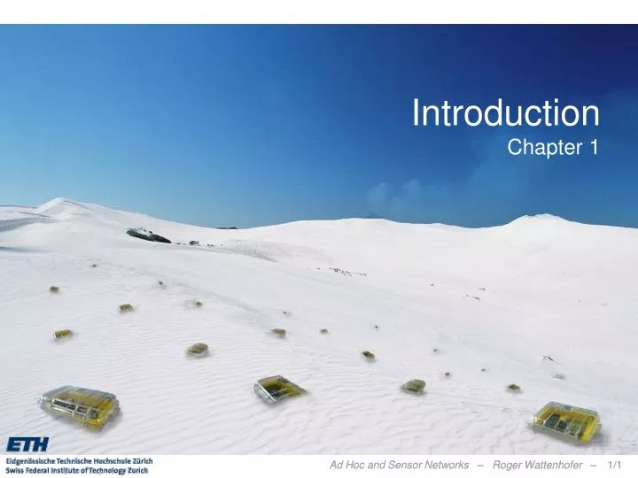
Introduction Chapter 1. Today, we look much cuter!. And we’re usually carefully deployed. Power. Radio. Processor. Sensors. Memory. A Typical Sensor Node: TinyNode 584. [ Shockfish SA, The Sensor Network Museum]. TI MSP430F1611 microcontroller @ 8 MHz

E N D
Today, we look much cuter! And we’re usually carefully deployed Power Radio Processor Sensors Memory
A Typical Sensor Node: TinyNode 584 [Shockfish SA, The Sensor Network Museum] • TI MSP430F1611 microcontroller @ 8 MHz • 10k SRAM, 48k flash (code), 512k serial storage • 868 MHz Xemics XE1205 multi channel radio • Up to 115 kbps data rate,200m outdoor range
After Deployment multi-hop communication
Laptops, PDA’s, cars, soldiers All-to-all routing Often with mobility (MANET’s) Trust/Security an issue No central coordinator Maybe high bandwidth Tiny nodes: 4 MHz, 32 kB, … Broadcast/Echo from/to sink Usually no mobility but link failures One administrative control Long lifetime Energy Ad Hoc Networks vs. Sensor Networks There is no strict separation; more variants such as mesh or sensor/actor networks exist
Overview • Introduction • Application Examples • Related Areas • Course Overview • Literature • For CS Students: Wireless Communication Basics • For EE Students: Network Algorithms Overview
Animal Monitoring (Great Duck Island) Biologists put sensors in underground nests of storm petrel And on 10cm stilts Devices record data about birds Transmit to research station And from there via satellite to lab
Environmental Monitoring (Redwood Tree) • Microclimate in a tree • 10km less cables on a tree; easier to set up • Sensor Network = The New Microscope?
Vehicle Tracking • Sensor nodes (equipped with magnetometers) are packaged, and dropped from fully autonomous GPS controlled “toy” air plane • Nodes know dropping order, and use that for initial position guess • Nodes thentrack vehicles(trucksmostly)
Park! Turn left! 30m to go… Turn right! 50m to go… Smart Spaces (Car Parking) • The good: Guide cars towards empty spots • The bad: Check which cars do not have any time remaining • The ugly: Meter running out: take picture and send fine [Matthias Grossglauser, EPFL & Nokia Research]
Structural Health Monitoring (Bridge) Detect structural defects, measuring temperature, humidity, vibration, etc. Swiss Made [EMPA]
Virtual Fence (CSIRO Australia) • Download the fence to the cows. Today stay here, tomorrow go somewhere else. • When a cow strays towards the co-ordinates, software running on the collar triggers a stimulus chosen to scare the cow away, a sound followed by an electric shock; this is the “virtual” fence. The software also "herds" the cows when the position of the virtual fence is moved. • If you just want to make sure that cows stay together, GPS is not really needed… Cows learn and need not to be shocked later… Moo!
Economic Forecast [Jean-Pierre Hubaux, EPFL] • Industrial Monitoring (35% – 45%) • Monitor and control production chain • Storage management • Monitor and control distribution • Building Monitoring and Control (20 – 30%) • Alarms (fire, intrusion etc.) • Access control • Home Automation (15 – 25%) • Energy management (light, heating, AC etc.) • Remote control of appliances • Automated Meter Reading (10-20%) • Water meter, electricity meter, etc. • Environmental Monitoring (5%) • Agriculture • Wildlife monitoring
RFID Systems • Fundamental difference between ad hoc/sensor networks and RFID: In RFID there is always the distinction between the passive tags/transponders (tiny/flat), and the reader (bulky/big). • There is another form of tag, the so-called active tag, which has its own internal power source that is used to power the integrated circuits and to broadcast the signal to the reader. An active tag is similar to a sensor node. • More types are available, e.g. the semi-passive tag, where the battery is not used for transmission (but only for computing)
Wearable Computing / Ubiquitous Computing • Tiny embedded “computers” • UbiComp: Microsoft’s Doll • I refer to my colleagueGerhard Troester andhis lectures & seminars [Schiele, Troester]
Wireless and/or Mobile • Aspects of mobility • User mobility: users communicate “anytime, anywhere, with anyone” (example: read/write email on web browser) • Device portability: devices can be connected anytime, anywhere to the network • Wireless vs. mobile Examples Stationary computer Notebook in a hotel Historic buildings; last mile Personal Digital Assistant (PDA) • The demand for mobile communication creates the need for integration of wireless networks and existing fixed networks • Local area networks: standardization of IEEE 802.11 or HIPERLAN • Wide area networks: GSM and ISDN • Internet: Mobile IP extension of the Internet protocol IP
Wireless & Mobile Examples • Up-to-date localized information • Map • Pull/Push • Ticketing • Etc. [Asus PDA, iPhone, Blackberry, Cybiko]
General Trend: A computer in 10 years? • Advances in technology • More computing power in smaller devices • Flat, lightweight displays with low power consumption • New user interfaces due to small dimensions • More bandwidth (per second? per space?) • Multiple wireless techniques • Technology in the background • Device location awareness: computers adapt to their environment • User location awareness: computers recognize the location of the user and react appropriately (call forwarding) • “Computers” evolve • Small, cheap, portable, replaceable • Integration or disintegration?
Physical Layer: Wireless Frequencies regulated 1 Mm 300 Hz 10 km 30 kHz 100 m 3 MHz 1 m 300 MHz 10 mm 30 GHz 100 m 3 THz 1 m 300 THz VLF LF MF HF VHF UHF SHF EHF infrared UV visible light twisted pair coax ISM AM SW FM
Frequencies and Regulations • ITU-R holds auctions for new frequencies, manages frequency bands worldwide (WRC, World Radio Conferences)
Course Overview 1 Applications 8 Clock Sync 9 Positioning 14 Transport 2 Geo-Routing 4 Data Gathering 13 Mobility 5 Network Coding 12 Routing 7 MAC Theory 6 MAC Practice 3 Topology Control 10 Clustering 1 Basics 11 Capacity Practice Theory
Course Overview: Lecture and Exercises • Maximum possible spectrum of theory and practice • New area, more open than closed questions • Each week, exactly one topic (chapter) • General ideas, concepts, algorithms, impossibility results, etc. • Most of these are applicable in other contexts • In other words, almost no protocols • Two types of exercises: theory/paper, practice/lab • Assistants: Philipp Sommer, Johannes Schneider • www.disco.ethz.ch courses
More Literature • BhaskarKrishnamachari – Networking Wireless Sensors • Paolo Santi – TopologyControl in Wireless Ad Hoc and Sensor Networks • F. Zhao and L. Guibas – Wireless Sensor Networks: An Information Processing Approach • Ivan Stojmeniovic – Handbook of Wireless Networks and Mobile Computing • C. SivaMurthy and B. S. Manoj – Ad Hoc Wireless Networks • Jochen Schiller – Mobile Communications • Charles E. Perkins – Ad-hoc Networking • Andrew Tanenbaum – Computer Networks • Plus tons of other books/articles • Papers, papers, papers, …
Rating (of Applications) • Area maturity • Practical importance • Theory appeal First steps Text book No apps Mission critical BoooooooringExciting
Open Problem • Well, the open problem for this chapter is obvious: • Find the killer application! Get rich and famous!! • …this lecture is only superficially about ad hoc and sensor networks. In reality it is about new (and hopefully exciting) networking paradigms!
For CS Students: Wireless Communication Basics • Brief history of communication • Frequencies • Signals • Antennas • Signal Propagation • Modulation
A brief history of communication • Electric telegraph invented in 1837 by Samuel Morse • First long distance transmission between Washington,D.C. and Baltimore, Maryland in 1844: «What hath God wrought» • Invention of the telephone by Alexander Graham Bell in 1875
Going Wireless • Guglielmo Marconi demonstrates first wireless telegraph in 1896. • A wireless telegraph service is established betweenFrance and England in 1898. • 1901 first wireless communication accross the atlantic • First amplitude modulation (AM) radio transmissionin 1906 • Edwin Howard Armstrong inventsfrequency modulation (FM) radio in 1935 • Digital Audio Broadcasting (DAB) since late 90’s
Wireless Telephony • First experiments with mobile phone systems in 1950s • Fully automated mobile phone system for vehicleslaunched in Sweden around 1960 • First generation (1G): cellular networks in Japan (1979) • Second generation (2G): GSM introduced in 1990sDigital network, SMS, roaming • Third generation (3G): high-speed data networks (UMTS)
Block Diagram of a Wireless Communication System • Modulation is required to transfer data over a wireless channel Transmitter Data In Modulator Antenna Wireless Channel Receiver Data Out Demodulator Antenna
Modulation and demodulation analog baseband signal digital data digital modulation analog modulation radio transmitter 101101001 radio carrier analog baseband signal digital data analog demodulation synchronization decision radio receiver 101101001 radio carrier • Modulation in action:
Periodic Signals • g(t) = At sin(2πft t + φt) • Amplitude A • frequency f [Hz = 1/s] • period T = 1/f • wavelength λwith λf = c (c=3∙108 m/s) • phase φ • φ* = -φT/2π[+T] A φ* t 0 T
Different representations of signals • For many modulation schemes not all parameters matter. A [V] I = A sin A [V] t [s] R = A cos * f [Hz] amplitude domain frequency spectrum phase state diagram
Digital modulation • Modulation of digital signals known as Shift Keying • Amplitude Shift Keying (ASK): • very simple • low bandwidth requirements • very susceptible to interference • Frequency Shift Keying (FSK): • needs larger bandwidth • Phase Shift Keying (PSK): • more complex • robust against interference 1 0 1 t 1 0 1 t 1 0 1 t
I R 1 0 I 11 10 R 00 01 Advanced Phase Shift Keying • BPSK (Binary Phase Shift Keying): • bit value 0: sine wave • bit value 1: inverted sine wave • Robust, low spectral efficiency • Example: satellite systems • QPSK (Quadrature Phase Shift Keying): • 2 bits coded as one symbol • symbol determines shift of sine wave • needs less bandwidth compared to BPSK • more complex
0010 I 0001 0011 0000 R 1000 Modulation Combinations • Quadrature Amplitude Modulation (QAM) • combines amplitude and phase modulation • it is possible to code n bits using one symbol • 2n discrete levels, n=2 identical to QPSK • bit error rate increases with n, but less errors compared to comparable PSK schemes • Example: 16-QAM (4 bits = 1 symbol) • Symbols 0011 and 0001 have the same phase, but different amplitude. 0000 and 1000 have different phase, but same amplitude. • Used in 9600 bit/s modems
Ultra-Wideband (UWB) • An example of a new physical paradigm. • Discard the usual dedicated frequency band paradigm. • Instead share a large spectrum (about 1-10 GHz). • Modulation: Often pulse-based systems. Use extremely short duration pulses (sub-nanosecond) instead of continuous waves to transmit information. Depending on application 1M-2G pulses/second
UWB Modulation • PPM: Position of pulse • PAM: Strength of pulse • OOK: To pulse or not to pulse • Or also pulse shape
Antennas: isotropic radiator • Radiation and reception of electromagnetic waves, coupling of wires to space for radio transmission • Isotropic radiator: equal radiation in all three directions • Only a theoretical reference antenna • Radiation pattern: measurement of radiation around an antenna • Sphere: S = 4π r2 z y Ideal isotropicradiator x
/2 Antennas: simple dipoles • Real antennas are not isotropic radiators but, e.g., dipoles with lengths /2 as Hertzian dipole or /4 on car roofs or shape of antenna proportional to wavelength • Example: Radiation pattern of a simple Hertzian dipole /4 z z y simple dipole x y x side view (xz-plane) side view (yz-plane) top view (xy-plane)
Antennas: directed and sectorized • Often used for microwave connections or base stations for mobile phones (e.g., radio coverage of a valley) z y directed antenna x/y x side (xz)/top (yz) views side view (yz-plane) [Buwal] y y sectorized antenna x x top view, 3 sector top view, 6 sector
Antennas: diversity • Grouping of 2 or more antennas • multi-element antenna arrays • Antenna diversity • switched diversity, selection diversity • receiver chooses antenna with largest output • diversity combining • combine output power to produce gain • cophasing needed to avoid cancellation • Smart antenna: beam-forming, MIMO, etc. /2 /2 /4 /2 /4 /2 + + ground plane
Signal propagation ranges, a simplified model • Propagation in free space always like light (straight line) • Transmission range • communication possible • low error rate • Detection range • detection of the signal possible • no communication possible • Interference range • signal may not be detected • signal adds to the background noise sender transmission distance detection interference
Signal propagation, more accurate models • Free spacepropagation • Two-raygroundpropagation • Ps, Pr: Power of radiosignal of sender resp. receiver • Gs, Gr: Antennagain of sender resp. receiver (how bad isantenna) • d: Distance betweensender and receiver • L: System lossfactor • ¸: Wavelength of signal in meters • hs, hr: Antennaheightaboveground of sender resp. receiver • Plus, in practice, received power is not constant („fading“)
Attenuation by distance • Attenuation [dB] = 10 log10 (transmitted power / received power) • Example: factor 2 loss = 10 log10 2 ≈ 3 dB • In theory/vacuum (and for short distances), receiving power is proportional to 1/d2, where d is the distance. • In practice (for long distances), receiving power is proportional to 1/d, α = 4…6.We call the path loss exponent. • Example: Short distance, what isthe attenuation between 10 and 100meters distance?Factor 100 (=1002/102) loss = 20 dB α = 2… 15-25 dB drop received power α = 4…6 LOS NLOS distance
Attenuation by objects • Shadowing (3-30 dB): • textile (3 dB) • concrete walls (13-20 dB) • floors (20-30 dB) • reflection at large obstacles • scattering at small obstacles • diffraction at edges • fading (frequency dependent) shadowing reflection scattering diffraction
Multipath propagation • Signal can take many different paths between sender and receiver due to reflection, scattering, diffraction • Time dispersion: signal is dispersed over time • Interference with “neighbor” symbols: Inter Symbol Interference (ISI) • The signal reaches a receiver directly and phase shifted • Distorted signal depending on the phases of the different parts signal at sender signal at receiver