Download
1 / 49
500 likes | 670 Views
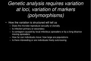
Genetic analysis requires variation at loci, variation of markers (polymorphisms). How the variation is structured will tell us Does the microbe reproduce sexually or clonally Is infection primary or secondary

E N D
Genetic analysis requires variation at loci, variation of markers (polymorphisms) • How the variation is structured will tell us • Does the microbe reproduce sexually or clonally • Is infection primary or secondary • Is contagion caused by local infectious spreaders or by a long-disance moving spreaders • How far can individuals move: how large are populations • Is there inbreeding or are individuals freely outcrossing
CASE STUDY • A grou A stand of adjacent trees is infected by a disease: How can we determine the way trees are infected?
CASE STUDY • A grou A stand of adjacent trees is infected by a disease: How can we determine the way trees are infected? BY ANALYSING THE GENOTYPE OF THE MICROBES: if the genotype is the same then we have local secondary tree-to-tree contagion. If all genotypes are different then primary infection caused by airborne spores is the likely cause of Contagion.
CASE STUDY • A grou WE HAVE DETERMINED AIRBORNE SPORES (PRIMARY INFECTION ) IS THE MOST COMMON FORM OF INFECTION QUESTION: Are the infectious spores produced by a local spreader, or is there a general airborne population of spores that may come from far away ? HOW CAN WE ANSWER THIS QUESTION?
If spores are produced by a local spreader.. • Even if each tree is infected by different genotypes (each representing the result of meiosis like us here in this class)….these genotypes will be related • HOW CAN WE DETERMINE IF THEY ARE RELATED?
HOW CAN WE DETERMINE IF THEY ARE RELATED? • By using random genetic markers we find out the genetic similarity among these genotypes infecting adjacent trees is high • If all spores are generated by one individual • They should have the same mitochondrial genome • They should have one of two mating alleles
WE DETERMINE INFECTIOUS SPORES ARE NOT RELATED • QUESTION: HOW FAR ARE THEY COMING FROM? ….or…… • HOW LARGE IS A POPULATION? Very important question: if we decide we want to wipe out an infectious disease we need to wipe out at least the areas corresponding to the population size, otherwise we will achieve no result.
HOW TO DETERMINE WHETHER DIFFERENT SITES BELONG TO THE SAME POP OR NOT? • Sample the sites and run the genetic markers • If sites are very different: • All individuals from each site will be in their own exclusive clade, if two sites are in the same clade maybe those two populations actually are linked (within reach) • In AMOVA analysis, amount of genetic variance among populations will be significant (if organism is sexual portion of variance among individuals will also be significant) • F statistics: Fst will be over ) 0.10 (suggesting sttong structuring) • There will be isolation by distance
Levels of Analyses • Individual • identifying parents & offspring– very important in zoological circles – identify patterns of mating between individuals (polyandry, etc.) • In fungi, it is important to identify the "individual" -- determining clonal individuals from unique individuals that resulted from a single mating event.
Levels of Analyses cont… • Families – looking at relatedness within colonies (ants, bees, etc.) • Population – level of variation within a population. • Dispersal = indirectly estimate by calculating migration • Conservation & Management = looking for founder effects (little allelic variation), bottlenecks (reduction in population size leads to little allelic variation) • Species – variation among species = what are the relationship between species. • Family, Order, ETC. = higher level phylogenies
What is Population Genetics? • About microevolution (evolution of species) • The study of the change of allele frequencies, genotype frequencies, and phenotype frequencies
Goals of population genetics • Natural selection (adaptation) • Chance (random events) • Mutations • Climatic changes (population expansions and contractions) • … To provide an explanatory framework to describe the evolution of species, organisms, and their genome, due to: Assumes that: • the same evolutionary forces acting within species (populations) should enable us to explain the differences we see between species • evolution leads to change in gene frequencies within populations
Pathogen Population Genetics • must constantly adapt to changing environmental conditions to survive • High genetic diversity = easily adapted • Low genetic diversity = difficult to adapt to changing environmental conditions • important for determining evolutionary potential of a pathogen • If we are to control a disease, must target a population rather than individual • Exhibit a diverse array of reproductive strategies that impact population biology
Analytical Techniques • Hardy-Weinberg Equilibrium • p2 + 2pq + q2 = 1 • Departures from non-random mating • F-Statistics • measures of genetic differentiation in populations • Genetic Distances – degree of similarity between OTUs • Nei’s • Reynolds • Jaccards • Cavalli-Sforza • Tree Algorithms – visualization of similarity • UPGMA • Neighbor Joining
Allele Frequencies • Allele frequencies (gene frequencies) = proportion of all alleles in an all individuals in the group in question which are a particular type • Allele frequencies: • p + q = 1 • Expected genotype frequencies: • p2 + 2pq + q2
Evolutionary principles: Factors causing changes in genotype frequency • Selection = variation in fitness; heritable • Mutation = change in DNA of genes • Migration = movement of genes across populations • Vectors = Pollen, Spores • Recombination = exchange of gene segments • Non-random Mating =mating between neighbors rather than by chance • Random Genetic Drift = if populations are small enough, by chance, sampling will result in a different allele frequency from one generation to the next.
The smaller the sample, the greater the chance of deviation from an ideal population. • Genetic drift at small population sizes often occurs as a result of two situations: the bottleneck effect or the founder effect.
Founder Effects; typical of exotic diseases • Establishment of a population by a few individuals can profoundly affect genetic variation • Consequences of Founder effects • Fewer alleles • Fixed alleles • Modified allele frequencies compared to source pop • GREATER THAN EXPECTED DIFFERENCES AMONG POPULATIONS BECAUSE POPULATIONS NOT IN EQUILIBRIUM (IF A BLONDE FOUNDS TOWN A AND A BRUNETTE FOUND TOWN B ANDF THERE IS NO MOVEMENT BETWEEN TOWNS, WE WILL ISTANTANEOUSLY OBSERVE POPULATION DIFFERENTIATION)
Bottleneck Effect • The bottleneck effect occurs when the numbers of individuals in a larger population are drastically reduced • By chance, some alleles may be overrepresented and others underrepresented among the survivors • Some alleles may be eliminated altogether • Genetic drift will continue to impact the gene pool until the population is large enough
Northern Elephant Seal: Example of Bottleneck Hunted down to 20 individuals in 1890’s Population has recovered to over 30,000 No genetic diversity at 20 loci
Hardy Weinberg Equilibriumand F-Stats • In general, requires co-dominant marker system • Codominant = expression of heterozygote phenotypes that differ from either homozygote phenotype. • AA, Aa, aa
Hardy-Weinberg Equilibrium • Null Model = population is in HW Equilibrium • Useful • Often predicts genotype frequencies well
Hardy-Weinberg Theorem if only random mating occurs, then allele frequencies remain unchanged over time. After one generation of random-mating, genotype frequencies are given by AA Aa aa p2 2pq q2 p = freq (A) q = freq (a)
Expected Genotype Frequencies • The possible range for an allele frequency or genotype frequency therefore lies between ( 0 – 1) • with 0 meaning complete absence of that allele or genotype from the population (no individual in the population carries that allele or genotype) • 1 means complete fixation of the allele or genotype (fixation means that every individual in the population is homozygous for the allele -- i.e., has the same genotype at that locus).
ASSUMPTIONS 1) diploid organism 2) sexual reproduction 3) Discrete generations (no overlap) 4) mating occurs at random 5) large population size (infinite) 6) No migration (closed population) 7) Mutations can be ignored 8) No selection on alleles
IMPORTANCE OF HW THEOREM If the only force acting on the population is random mating, allele frequencies remain unchanged and genotypic frequencies are constant. Mendelian genetics implies that genetic variability can persist indefinitely, unless other evolutionary forces act to remove it
Departures from HW Equilibrium • Check Gene Diversity = Heterozygosity • If high gene diversity = different genetic sources due to high levels of migration • Inbreeding - mating system “leaky” or breaks down allowing mating between siblings • Asexual reproduction = check for clones • Risk of over emphasizing particular individuals • Restricted dispersal = local differentiation leads to non-random mating
Pop 3 Pop 2 Pop 1 Pop 4 FST = 0.30 FST = 0.02
Local Inbreeding Coefficient • Calculate HOBS • Pop1: 4/20 = 0.20 • Pop2: 10/20 = 0.50 • Pop3: 8/20 = 0.40 • Calculate HEXP(2pq) • Pop1: 2*0.60*0.40 = 0.48 • Pop2: 2*0.50*0.50 = 0.50 • Pop3: 2*0.20*0.80 = 0.32 • Calculate F = (HEXP – HOBS)/ HEXP • Pop1 = (0.48 – 0.20)/(0.48) = 0.583 • Pop2 = (0.50 – 0.50)/(0.50) = 0.000 • Pop3 = (0.32 – 0.40)/(0.32) = -0.250
F StatsProportions of Variance • FIS = (HS – HI)/(HS) • FST = (HT – HS)/(HT) • FIT = (HT – HI)/(HT)
Important point • Fst values are significant or not depending on the organism you are studying or reading about: • Fst =0.10 would be outrageous for humans, for fungi means modest substructuring
Microsatellites or SSRs • AGTTTCATGCGTAGGT CG CG CG CG CG AAAATTTTAGGTAAATTT • Number of CG is variable • Design primers on FLANKING region, amplify DNA • Electrophoresis on gel, or capillary • Size the allele (different by one or more repeats; if number does not match there may be polimorphisms in flanking region) • Stepwise mutational process (2 to 3 to 4 to 3 to2 repeats)
Host islands within the California Northern Channel Islands create fine-scale genetic structure in two sympatric species of the symbiotic ectomycorrhizal fungus Rhizopogon Rhizopogon occidentalis Rhizopogon vulgaris
Rhizopogon sampling & study area • Santa Rosa, Santa Cruz • R. occidentalis • R. vulgaris • Overlapping ranges • Sympatric • Independent evolutionary histories
Local Scale Population StructureRhizopogon occidentalis FST = 0.26 8-19 km N E 5 km FST = 0.33 FST = 0.24 W B T FST = 0.17 Populations are similar Populations are different Grubisha LC, Bergemann SE, Bruns TD Molecular Ecology in press.
Local Scale Population StructureRhizopogon vulgaris FST = 0.21 N E FST = 0.25 FST = 0.20 W Populations are different Grubisha LC, Bergemann SE, Bruns TD Molecular Ecology in press