Download
1 / 29
300 likes | 335 Views
Learn about single-source and all-pair shortest path algorithms, including Bellman-Ford and Dijkstra. Understand optimal substructure, shortest path properties, and the Floyd-Warshall algorithm for weighted graphs.

E N D
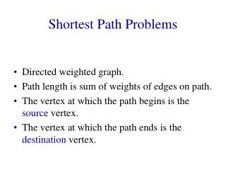
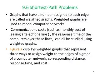
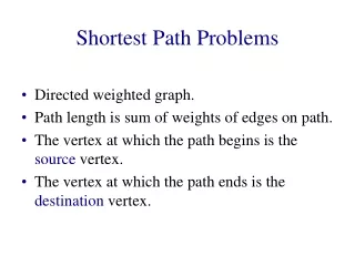
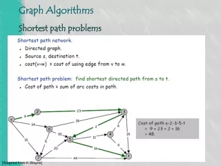
Lecture 7 Shortest Path • Shortest-path problems • Single-source shortest path • All-pair shortest path
Overview • Shortest-path problems • Single-source shortest path algorithms • Bellman-Ford algorithm • Dijkstra algorithm • All-Pair shortest path algorithms • Floyd-Warshall algorithm
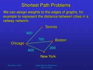
Weighted graph Beijing Qingdao Lhasa Shanghai • Single-source shortest path • All-pair shortest path Guangzhou
Shortest Path Optimal substructure: Subpaths of shortest paths are shortest paths. Cycles. Can a shortest path contains cycles? Negative weights.
Where are we? • Shortest-path problems • Single-source shortest path algorithms • Bellman-Ford algorithm • Dijkstra algorithm • All-Pair shortest path algorithms • Floyd-Warshall algorithm
Relaxing The process of relaxingan edge (u,v)consists of testing whether we can improve the shortest path to vfound so far by going through u.
Shortest-path properties Notation: We fix the source to be s. λ[v]: the length of path computed by our algorithms from s to v. δ[v]: the length of the shortest path from s to v. Triangle property δ[v] <= δ[u] + w(u,v) for any edge (u,v). Upper-bound property δ[v] <= λ[v] for any vertex v. Convergence property If s⇒u→v is a shortest path, and if λ[u] = δ[u], then after relax(u,v), we have λ[v] = δ[v].
Θ(mn) Bellman-Ford algorithm E = {(t,x),(t,y),(t,z),(x,t),(y,x),(y,z),(z,x),(z,s),(s,t),(s,y)}
Quiz Run Bellman-Ford algorithm for the following graph, provided by E = {(S,A),(S,G),(A,E),(B,A),(B,C),(C,D),(D,E),(E,B),(F,A),(F,E),(G,F)}
Proof. No negative cycle. By the fact that the length of simple paths is bounded by |V| - 1. After i-th iteration of relax, λ[vi] = δ[vi]. s v1 vj vi v Correctness Correctness of Bellman-Ford If G contains no negative-weight cycles reachable from s, then the algorithm returns TRUE, and for all v, λ[v] = δ[v], otherwise the algorithm returns FALSE. Negative cycle. Assume vj,…, vi, vj. is a negative cycle and assume Bellman-Ford returns TRUE. λ[vk+1] <= λ[vk] + w(vk,vk+1) Sum all the inequalities together, we will get controdictions.
s v1 vj vi v • Θ(m) Observation 1 If there is no cycle (DAG), ... Relax in topological order.
seam Weighted DAG application
Observation 2 If there is no negative edge, ... vj vi v1 s If (s, vi) is the lightest edge sourcing from s, then λ[vi] = δ[vi]
Dijkstra algorithm Edsger Wybe Dijkstra in 2002
Correctness Assume u is chosen in Step 7, and 1. λ[u] > δ[u] 2. s ⇒ x → y ⇒ u is the shortest path δ[u] = δ[x] + w(x,y) + w(p2) = λ[x] + w(x,y) + w(p2) ≥ λ[x] + w(x,y) ≥ λ[y] ≥ λ[u]
Θ(n2) Time complexity
What is the time complexity? • How about use d-heap?
Dense graph • dense: m = n1+ε, ε is not too small. • d-heap, d = m/n • complexity: O(dnlogdn + mlogdn) = O(m)
Where are we? • Shortest-path problems • Single-source shortest path algorithms • Bellman-Ford algorithm • Dijkstra algorithm • All-Pair shortest path algorithms • Floyd-Warshall algorithm
Θ(n3) Floyd-Warshall algorithm
Quiz Run Floyd-Warshall algorithm for the following graph:
Conclusion Dijkstra’s algorithm. • Nearly linear-time when weights are nonnegative. Acyclic edge-weighted digraphs. • Faster than Dijkstra’s algorithm. • Negative weights are no problem. Negative weights and negative cycles. • If no negative cycles, can find shortest paths via Bellman-Ford. • If negative cycles, can find one via Bellman-Ford. All-pair shortest path. • can be solved via Floyd-Warshall • Floyd-Warshall can also compute the transitive closure of directed graph.