Download
1 / 39
400 likes | 583 Views
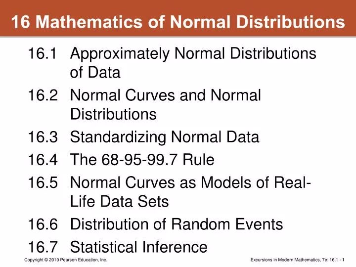
16 Mathematics of Normal Distributions. 16.1 Approximately Normal Distributions of Data 16.2 Normal Curves and Normal Distributions 16.3 Standardizing Normal Data 16.4 The 68-95-99.7 Rule 16.5 Normal Curves as Models of Real-Life Data Sets 16.6 Distribution of Random Events

E N D
16 Mathematics of Normal Distributions 16.1 Approximately Normal Distributions of Data 16.2 Normal Curves and Normal Distributions 16.3 Standardizing Normal Data 16.4 The 68-95-99.7 Rule 16.5 Normal Curves as Models of Real-Life Data Sets 16.6 Distribution of Random Events 16.7 Statistical Inference
Example 16.1 Distribution of Heights of NBA Players This table is a frequency table giving the heights of 430 NBA players listed onteam rosters at the start of the 2008–2009 season.
Example 16.1 Distribution of Heights of NBA Players The bar graph for this data setis shown.
Example 16.2 2007 SAT Math Scores The table on the next slide shows the scores of N = 1,494,531 college-bound seniors on the mathematics section of the 2007 SAT. (Scores range from 200 to 800 and are groupedin class intervals of 50 points.) The table shows the score distribution and the percentage of test takers in each class interval.
Example 16.2 2007 SAT Math Scores Here is a bar graph of the data.
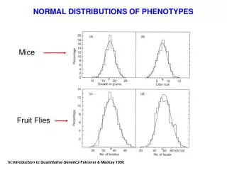
Approximately Normal Distribution The two very different data sets haveone thing in common–both can be described as having bar graphs that roughlyfit a bell-shaped pattern. These data sets have an approximately normaldistribution.
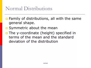
Normal Distribution A distribution of data that has a perfect bell shape is called a normaldistribution.
Normal Curves Perfect bell-shaped curves are called normal curves. Every approximatelynormal data set can be idealized mathematically by a corresponding normalcurve This is important because wecan then use the mathematical properties of the normal curve to analyze anddraw conclusions about the data.
Normal Curves Some bells are short and squat,others are tall and skinny, andothers fall somewhere in between.
Essential Facts About Normal Curves Symmetry. Every normal curve has a vertical axis of symmetry, splitting the bell-shaped region outlined by the curve into two identicalhalves. This is the only line of symmetry of a normal curve.
Essential Facts About Normal Curves Median / mean. We will call the point of intersection of the horizontalaxis and the line of symmetry of the curve the center of the distribution.
Essential Facts About Normal Curves Median / mean. The center represents both the medianM and themean (average) of the data. In a normal distribution, M = . The fact that in a normal distribution the median equals the mean implies that 50% of the data are less than or equal to the mean and 50%of the data are greater than or equal to the mean.
MEDIAN AND MEAN OF A NORMAL DISTRIBUTION In a normal distribution, M = . (If the distribution is approximately normal,then M ≈ .)
Essential Facts About Normal Curves Standard Deviation. The standard deviation is an important measure of spread, and it is particularly useful when dealing with normal (or approximately normal) distributions.– Denoted by theGreek letter called sigma
Essential Facts About Normal Curves Standard Deviation. If you wereto bend a piece of wire into a bell-shaped normal curve, at the very top you would be bending the wire downward.
Essential Facts About Normal Curves Standard Deviation. But, at the bottom you would be bending the wire upward.
Essential Facts About Normal Curves Standard Deviation. As you move your handsdown the wire, the curvature gradually changes, and there is one point oneach side of the curve where the transition from being bent downward tobeing bent upward takes place. Such a point is called apoint of inflection of the curve.
Essential Facts About Normal Curves Standard Deviation. The standard deviation of a normal distribution is the horizontal distance between the line of symmetry of the curve and one of the two points of inflection, P´ or P in the figure.
STANDARD DEVIATION OF A NORMAL DISTRIBUTION In a normal distribution, the standard deviation equals the distance betweena point of inflection and the line of symmetry of the curve.
Essential Facts About Normal Curves Quartiles. We learned in Chapter 14 how to find the quartiles of a data set. When the data set has a normal distribution, the first and third quartilescan be approximated using the mean and the standard deviation . Multiplying the standard deviation by0.675 tells us how far to go to the right or left of the mean to locate thequartiles.
QUARTILES OF A NORMAL DISTRIBUTION In a normal distribution, Q3 ≈ + (0.675) and Q1 ≈ – (0.675). Pg. 604 # 6
Standardizing the Data We have seen that normal curves don’t all look alike, but this is only a matter ofperception. All normal distributions tell the same underlying story but useslightly different dialects to do it. One way to understand the story of any givennormal distribution is to rephrase it in a simple languagethat uses the mean and the standard deviation as its only vocabulary. Thisprocess is called standardizing the data.
z-value To standardize a data value x, we measure how far x has strayed from themean using the standard deviation as the unit of measurement. A standardizeddata value is often referred to as a z-value. The best way to illustrate the process of standardizing normal data is bymeans of a few examples.
Example 16.4 Standardizing Normal Data Let’s consider a normally distributed data set with mean = 45ft and standarddeviation = 10 ft. We will standardize several data values, starting with a couple of easy cases.
Example 16.4 Standardizing Normal Data ■x4 = 21.58 is ... uh, this is a slightly more complicated case. How do we handle this one? First, we find the signed distance between the data value andthe mean by taking their difference (x4– ). In this case we get 21.58 ft –45 ft= –23.42 ft.(Notice that for data values smaller than the mean this difference will be negative.)
Example 16.4 Standardizing Normal Data ■If we divide this difference by = 10 ft, we get the standardized valuez4= –2.342. This tells us the data point x4 is –2.342 standard deviations from the mean = 45 ft (D in the figure).
STANDARDING RULE In a normal distribution with mean and standard deviation , the standardizedvalue of a data point x is z = (x – )/. Pg. 605 # 18a,b,
Standardizing Normal Data One important point to note is that while the original data is given with units,there are no units given for the z-value. The units for the z-value are standarddeviations, and this is implicit in the very fact that it is a z-value.
Finding the Value of a Data Point The process of standardizing data can also be reversed, and given a z-valuewe can go back and find the corresponding x-value. To do this take theformulaz = (x – )/ and solve for x in terms of z. x = + •z Pg. 605 # 22a,c Groups Pg. 604 #4d, 8, 18c,d, 22b,d, 25
The 68-95-99.7 Rule In a typical bell-shaped distribution, most of thedata are concentrated near the center. As we move away from the center theheights of the columns drop rather fast, and if we move far enough away from thecenter, there are essentially no data to be found.
The 68-95-99.7 Rule These are all rather informal observations, but there is a more formal way to phrase this, called the 68-95-99.7rule. This useful rule is obtained by using one, two, and three standard deviationsabove and below the mean as special landmarks. In effect, the 68-95-99.7 rule isthree separate rules in one.
THE 68-95-99.7 RULE • In every normal distribution, about 68% of all the data values fall within onestandard deviation above and below the mean. In other words, 68% of all thedata have standardized values between z = –1 and z = 1.
THE 68-95-99.7 RULE 2. In every normal distribution, about 95% of all the data values fall within twostandard deviations above and below the mean. In other words, 95% of all thedata have standardized values between z = –2 and z = 2.
THE 68-95-99.7 RULE 3. In every normal distribution, about 99.7% (i.e., practically 100%) of all the data values fall within threestandard deviations above and below the mean. In other words, 99.7% of all thedata have standardized values between z = –3 and z = 3.
Practical Implications Earlier in the text, we defined the range R of a data set (R = Max – Min) and, in the case of an approximately normal distribution, we can conclude thatthe range is about six standard deviations. This is true as long aswe can assume that there are no outliers. Pg. 606 # 32a, 34, 42, 52c Groups # 34, 44a,d, 52a,b,d,e