Particle Filter Based Traffic State Estimation Using Cell Phone Network Data
240 likes | 374 Views
Particle Filter Based Traffic State Estimation Using Cell Phone Network Data. Peng Cheng, Member, IEEE, Zhijun Qiu , and Bin Ran Presented By: Guru Prasanna Gopalakrishnan. Overview. Background- Where it fits? Problem Formulation Traffic Models First Order Traffic Model

Particle Filter Based Traffic State Estimation Using Cell Phone Network Data
E N D
Presentation Transcript
Particle Filter Based Traffic State Estimation Using Cell PhoneNetwork Data Peng Cheng, Member, IEEE, ZhijunQiu, and Bin Ran Presented By: Guru PrasannaGopalakrishnan
Overview • Background- Where it fits? • Problem Formulation • Traffic Models • First Order Traffic Model • Second Order Traffic Model • Particle Filter Design • Experimental Results • Conclusion
Introduction-I • Traffic time and congestion information valued by road users and road system managers1 • Applications- Incident detection, Traffic management, Traveler information, Performance monitoring • Two approaches to collect real-time traffic data - Fixed Sensors - Mobile Sensors
Introduction-II • Fixed Sensor System - Inductive loops, Radar, etc - Real-time information collection - Dense Sampling technique • Mobile Sensor System • Handset Based Solutions • Network Based Solutions • Sparse Sampling Technique
Problem Formulation- I • Key Points: • Microcells of similar size • - Randomization of Handoff points
Problem Formulation II Definitions: - H=(IDcell phone, thandoff, Cellfrom, Cellto) • - Handoff pair
Traffic Model • Traffic flow modeled as stochastic dynamic system with discrete-time states • State Variable: - xi,k= {Ni,k , i,k}T • Generic model of system state evolution - xk+1=fk(xk, wk) - fk is system transition function and wk is the system noise - yk=hk(xk, k) - hkis measurement function and k measurement error
Important Terminologies • Ni,k-Number of vehicles in section I at sampling time tk • i,k-Average speed of the vehicles • Q,i,k - number of vehicles crossing the cell boundary from link i to link i+1 during the time interval k • i,k, - Constant and scale co-efficient respectively • i,t ,e - Intermediate speed and equilibrium speed • i,t , crit- Anticipated traffic density and critical density • Si,t, Ri+1,t-Sending and Receiving functions respectively
First-order Traffic Model • Traffic speed is the only state variable • System State Equation: • i,k+1=i,ki-1,k+i,ki,k+i,ki+1,k+ wi,ki=1,2,3,….n • Measurement Equation: • yi,k= avgi,k+k i=1,2,3,….n - avgi,k= Li/(tj+-tj-) - For stable road-traffic, i,k+ i,k+i,k=1
Second Order Traffic Model-I • Traffic volume is the second state variable • Macroscopic level- System State Equation: • Qi,k+1= Ui,t + W1i,k • Vi,k+1= (1/ Ʈk) i,t+ w2i,ki=1,2…n; k=1,2,….K • Macroscopic level- Measurement Equation: • Y1i,k = (1/i,k) Qi,k . e-Li/vi,k+ 1i,k • Y2i,k= Vi,k+2i,ki=1,2…n; k=1,2,….K • Note: • Ni,k+1=Ni,k+ Qi-1,k-Qi,k
Second Order Traffic Model-II • Microscopic System State Equation: • Ni,t+1=Ni,t+ Ui-1,t-Ui,t • i,t+1= i,t+1 +(1- )e(i,t+1) + w3i,t [0,1] Where - i,t+1 = { (i-1,t Qi-1,t + i,t(Ni,t- Qi,t))/Ni,t+1 Ni,t+1K0 { free o.w - i,t+1 = i,t+1 +(1-)i+1,t+1 [0,1] - Ni,t= i,t.Li i=1,2,…n
Second Order Traffic Model-III • Microsocopic System State Equation Contd… - e()={free.e-(0.5)(/crit)3.5if <=crit { free.e-(0.5)(- crit) Otherwise - Ui,t = min(Si,t , Ri,t+1) - Si,t= max(Ni,t.(i,tt)/Li + W4i,t, Ni,t (Vout,min t)/Li ) - Ri+1,t=(Li+1.l/Al)+Ui+1,t- Ni+1,t
State Transition and Reconstruction Y1i,k Y1i,k+1 Y2i,k Y2i,k+1 State Transition Macroscopic Level Microscopic level State Reconstruction Qi,k Vi,k ,t Qi,k+1 Vi,k+1 ,t Ui,1 i,1 Ui,2 i,2 Ui,3 i,3 Ui,k i,Ʈk
Particle Filter- Why? I • Bayesian estimation to construct conditional PDF of the current state xk given all available information Yk= {yj j=1,2,…..k} • Two steps used in construction of p(xk/Yk) 1) Prediction p(xk/Yk-1)=fp(xk/Xk-1) p(xk-1/Yk-1) dxk-1 and 2) Updation p(xk/Yk)= p(Yk/Xk) p(xk-1/Yk-1) / p(Yk/Yk-1)
Particle Filter-Why? II • p(Yk/Yk-1) – A normalized constant • p(xk/Xk-1)= fc(xk-fk-1(Xk-1, Wk-1))p(Wk-1) dwk-1 - p(Wk) is PDF of noise term in system equation • p(Yk/Xk)= fc(Yk-hk(Xk,k))p( k) d k - p( k) is PDF of noise term in measurement equation - c(.) is dirac delta function
Particle Filter- Why? III • No Simple analytical solution for p(xk/Yk) • Particle filter is used to find an approximate solution by empirical histogram corresponding to a collection of M particles
Particle Filter Implementation-I • Step 1: Initialization • For l=1,2,….M , Sample x0(l) ~ p(x0) q0= 1/M set K=1 • Step 2: Prediction • For l=1,2,….M , Sample xk(l) ~ p(xk/xk-1) • Step 3: Importance Evaluation • For l=1,2,….M , qk= (p(yk /xk) q(l)k-1/ ( p(yk /x(j)k) q(j)k-1
Particle Filter Implementation-II • Selection - Multiple/suppress M particles {xk(l)} according to their importance weights and obtain new M unweighted particles. • Output • P(xk/Yk)= qk(l).c(xk-xk(l)) • Posterior mean, xk=E(xk/Yk)=(1/M ) xk(l) • Posterior Co-Variance, V(xk/Yk)=(1/(M-1) ) (xk(l)-xk) (xk(l)-xk)T • Last Step - Let k=k+1 and Goto Step-2
Conclusion • Implemented using an existing infrastructure • Some Critiques • Interference due to parallel freeways2 • Cannot differentiate between pedestrians and moving vehicles • Some Unrealistic assumptions
References • G. Rose, Mobile phones as traffic probes, Technical Report, Institute of Transportation Studies, Monash University, 2004 • L. Mihaylova and R. Boel, “A Particle Filter for Freeway Traffic Estimation,” Proc. of 43rd IEEE Conference on Decision and Control, Vol. 2, pp. 2106 - 2111, 2004.