Download
1 / 18
180 likes | 214 Views
Learn about landmark comparison, restricted mean survival time, Mantel-Haenszel Test, interpreting differences in survival curves, and more. Explore examples and references in statistical analysis for medical studies.

E N D
Comparison of Two Survival Curves Landmark comparison at a pre-specified time t: divide S^T(t) – S^C(t) by the standard error of the difference computed using Greenwood’s estimator. See “Point-by-Point” Comparisons, p. 329 of FFDRG. Chappell – BMI 542, Spring 2018 These slides come after the Kaplan-Meier Mechanics .pdf and before the slides on biasing the Kaplan-Meier.
A reminder: What’s the simplest way to test whether an unknown quantity “Q” is equal to “17”? Estimate Q with Q^ Estimate its standard deviation, SE^(Q^) Then under H0 [Q^ - 17]/SE^(Q^) should be N(0,1) Equivalently, [Q^ - 17]2/Var^(Q^) should be X2(1) (Remember that the Var = SE2). We often use this to test that differences are 0. (This is very similar to a two-sample t-test.)
What about multiple unknown quantities? How do we test whether quantities Q1, Q2, … are equal to 17, 18, …? Same as before but add up numerators and denominators (variances only, not standard deviations): Estimate Q1, Q2, … with say Q1^, Q2^, … We assume that these estimates are independent. Estimate their variances Var^(Q1^), Var^(Q2^), … Then under H0 [Q1^ - 17) + (Q2^ - 18) + …]2/ [Var^(Q1^), Var^(Q2^), + …] is distributed X2(1) (or its square root is N(0,1).
How do we test that one unknown, Q1, equals another, Q2? Estimate Q1 with Q1^ and Q2 with Q2^ Estimate their variances with Var^(Q1^) and Var^(Q2^). Then under H0 [Q1^ - Q2^]/sqrt[Var^(Q1^) + Var^(Q2^)] should be N(0,1) (This is very similar to a two-sample t-test.)
Comparison of Two Survival Curves • 2. Restricted mean survival time (= RM life) at time t: • Mean survival up to time t; • = Mean[min(t, survival time)] • = Area under S^(.) between 0 and t. • Interpreted as “Mean number of years lived out of t” • Not “Mean number of years lived given death before t”: what is the RMST(5 years) for US newborns? • Can also be added & subtracted, as with unrestricted means, e.g.: • RMOverallSurvivalT(3 years) = • RMTto recurrence(3) + RMTfromRecurrencetoDeath(3)
Comparison of Two Survival Curves • 2. Restricted mean survival time (cont.): • Not in FFDRG, but see Uno, et al., “Alternatives to hazard ratios for comparing efficacy or safety of therapies in noninferiority studies.” Ann Intern Med. 163, pp. 127-134: 2015 for references and examples in diabetes and colorectal cancer. • See Glasziou, Simes, & Gelber, Stat. in Med. 9, 1259-1276: 1990 for an example in breast cancer. • For short description of general considerations, see Chappell & Zhu, “Describing differences in survival curves.” JAMA Onc., published online 4/28/2016.
Comparison of Two Survival Curves • 3. Mantel-Haenszel (Log-rank) Test • Ref: Mantel & Haenszel (1959) J Natl Cancer Inst • Mantel (1966) Cancer Chemotherapy Reports • - Mantel and Haenszel (1959) showed that a series of 2 x 2 • tables could be combined into a summary statistic, based on the work of Cochran and Cox. • - Mantel (1966) applied this procedure to the comparison of • two survival curves. • - Basic idea is to form a 2 x 2 table at each distinct death time, determining the number in each group who were at • risk and number who died.
Suppose we have K distinct times for a death occurring at • tj j = 1,2, .., K. • For each death time tj, we have a table such as on p. 330 of FFDRG. They use standard “contingency table notation”. To translate into “survival analysis notation”: • DjI = # of deaths at time tj in Intervention group = aj • DjC = # of deaths at time tj in Control group = cj • RjI = # at risk at time tj in Intervention group = aj + bj • RjC = # at risk at time tj in Control group = cj + dj . • See table on p. 330 of FFD. • Consider aj, the observed number of • deaths in the TRT group, under H0
Remember: “What about multiple unknown quantities?” How do we test whether quantities Q1, Q2, … are equal to 17, 18, …? Same as before but add up numerators and denominators (variances only, not standard deviations): Estimate Q1, Q2, … with say Q1^, Q2^, … We assume that these estimates are independent. Estimate their variances Var^(Q1^), Var^(Q2^), … Then under H0 [Q1^ - 17) + (Q2^ - 18) + …]2/ [Var^(Q1^), Var^(Q2^), + …] is distributed X2(1).
To translate into our current notation: Instead of: “How do we test whether quantities Q1, Q2, … are equal to 17, 18, …?” We use the numbers of deaths in Group 1 at each failure time: “How do we test whether, at each failure time tj, we have the observed number of deaths aj equal to the expected, E(aj)?” We add up the small pieces of information at each failure time.
E(aj) = (aj + bj)(aj + cj)/Ni Mantel-Haenszel Statistic
Table 15.3: Comparison of Survival Data for a Control Group and an Intervention Group Using the Mantel-Haenszel Procedure Rank Event Intervention Control Total Times j tj aj + bj ajlj cj + dj cjlj aj + cj bj + dj 1 0.5 20 0 0 20 1 1 1 39 2 1.0 20 1 0 18 0 0 1 37 3 1.5 19 0 2 18 2 1 2 35 4 3.0 17 0 1 15 1 2 1 31 5 4.5 16 1 0 12 0 0 1 27 6 4.8 15 0 1 12 1 0 1 26 7 6.2 14 0 1 11 1 2 1 24 8 10.5 13 0 1 8 1 1 20 • aj + bj = number of subjects at risk in the intervention group prior to the death at time tj • cj + cj = number of subjects at risk in the control group prior to the death at time tj • aj = number of subjects in the intervention group who died at time tj • cj = number of subjects in the control group who died at time tj • lj = number of subjects who were lost or censored between time tj and time tj+1 • aj + cj = number of subjects in both groups who died at time tj • bj + dj = number of subjects in both groups who are at risk minus the number who died at time tj
Mantel-Haenszel Test • Operationally • 1. Rank event times for both groups combined • 2. For each failure, form the 2 x 2 table • a. Number at risk (ai + bi, ci + di) • b. Number of deaths (ai, ci) • c. Losses (lTi, lCi) • Example (See Table 15-3 FFDRG) - Use previous data set • Trt: 1.0, 1.6+, 2.4+, 4.2+, 4.5, 5.8+, 7.0+, 11.0+, 12.0+'s • Control: 0.5, 0.6+, 1.5, 1.5, 2.0+, 3.0, 3.5+, 4.0+, 4.8, 6.2, • 8.5+, 9.0+, 10.5, 12.0+'s
1. Ranked Failure Times - Both groups combined 0.5, 1.0, 1.5, 3.0, 4.5, 4.8, 6.2, 10.5 C T C C T C C C 8 distinct times for death (k = 8) 2. At t1 = 0.5 (k = 1) T: a1 + b1 = 20 a1 = 0 lT1 = 0 c1 + d1 = 20 c1 = 1 lC1 = 1 D A R T 0 20 20 C 1 19 20 1 39 40 E(a1)= 1•20/40 = 0.5 V(a1) = 1•39 • 20 • 20 402 •39
E(a2)= 1•20 38 V(a2) = 1•37 • 20 • 18 382 •37 3. At t2 = 1.0 (k = 2) T: a2 + b2 = (a1 + b1) - a1 - lT1 a2 = 1.0 = 20 - 0 - 0 = 20 lT2 = 3 C. c2 + d2 = (c1 + d1) - c1 - lC1 c2 = 0 = 20 - 1 - 1 = 18 lC2 = 0 so D A R T 1 19 20 C 0 18 18 1 37 38
Eight 2x2 Tables Corresponding to the Event TimesUsed in the Mantel-Haenszel Statistic in Survival Comparison of Treatment (T) and Control (C) Groups 1. (0.5 mo.)* D† A‡ R§ 5. (4.5 mo.)* D A R T 0 20 20 T 1 15 16 C 1 19 20 C 0 12 12 1 39 40 1 27 28 2. (1.0 mo) D A R 6. (4.8 mo.) D A R T 1 19 20 T 0 15 15 C 0 18 18 C 1 11 12 1 37 38 1 26 27 3. (1.5 mo.) D A R 7. (6.2 mo.) D A R T 0 19 19 T 0 14 14 C 2 16 18 C 1 10 11 2 35 37 1 24 25 4. (3.0 mo.) D A R 8. (10.5 mo.) D A R T 0 17 17 T 0 13 13 C 1 14 15 C 1 7 8 1 31 32 1 20 21 * Number in parentheses indicates time, tj, of a death in either group † Number of subjects who died at time tj ‡ Number of subjects who are alive between time tj and time tj+1 § Number of subjects who were at risk before the death at time tj R=D+A)
Compute MH Statistics Recall K = 1 K = 2 K = 3 t1 = 0.5 t2 = 1.0 t3 = 1.5 D A 0 20 20 1 19 20 1 39 40 D A 1 19 20 0 18 18 1 37 38 D A 0 19 19 2 16 18 2 35 37 a. ai = 2 (only two treatment deaths) b. E(ai ) = 20(1)/40 + 20(1)/38 + 19(2)/37 + . . . = 4.89 c. V(ai) = = 2.22 d. MH = (2 - 4.89)2/2.22 = 3.76 or ZMH =
Comparison of Two Survival Curves 4. Peto (old-fashioned version: Gehan) modification of the Wilcoxon Test to account for censored data. • Derived as a modification of the Wilcoxon two-sample rank test. • Equivalent to a weighted MH (logrank) test, with the weight at time tj = S^(tj), the Kaplan-Meier curve for the combined sample. • When would we want to use decreasing weights? • When (if ever) would we want to use increasing weights?