Download
1 / 43
440 likes | 668 Views
Hydroinformatics for MSc in Environmental Engineering and Hydrology http://www3.imperial.ac.uk/ewre/courses/mschydrology/hydroinformatics/. Learning GIS (#8) Learning ArcGIS Spatial Analyst http://tinyurl.com/hydroinformatics. Ivan Stoianov ivan.stoianov@imperial.ac.uk (Room 328B)

E N D
Hydroinformatics for MSc in Environmental Engineering and Hydrologyhttp://www3.imperial.ac.uk/ewre/courses/mschydrology/hydroinformatics/ Learning GIS (#8) Learning ArcGIS Spatial Analyst http://tinyurl.com/hydroinformatics Ivan Stoianov ivan.stoianov@imperial.ac.uk (Room 328B) Environmental and Water Resources Engineering Section Imperial College December, 2008
Learning Objectives • understand how ArcGIS Spatial Analyst fits into the geoprocessing framework • set up an analysis environment • run Spatial Analyst operations • convert between feature and raster data • reclassify data
Exercise 1: Estimate tornado damagewww.tinyurl.com/hydroinformatics
- Buffering- Overlaying- Geo-processing- Spatial Analyst Analysis of Spatial Data
Input Raster Output Extent Output Cell Size Mask Output raster
ArcGIS SPATIAL ANALYST • ArcGIS Spatial Analyst allows us to perform tasks such as: • Surface analysis – how steep is a location? • Surface creation – a DEM from points. • Raster calculation – helps combine different data (map algerbra) • Distance Analysis – what is the shortest distance between two locations.
Surface Analysis • Surface Analysis tools derive useful geospatial information from elevation surfaces such as • Slope • Aspect • Hillshade • Viewshed
Exercise 2: Work with Spatial Analyst tools www.tinyurl.com/hydroinformatics (Scroll to Lecture 8) Download and unzip (Exercises & Description of Exercises) Note: a new folder was created under: C:\GIS_Course\Lesson2
Preparing data for analysis • organize your workspaces • determine the tools you need • identify data required for your analysis • convert vector to raster • reclassify data
Exercise #3 Convert vector data to raster data
Reclassify raster data Reclassification is the process of reassigning a value, arrange of values, or a list of values in a raster to new output values. Why reclassify: One reason is to set specific values to NoData to exclude them from analysis. Other reasons are to change values in response to new information or classification schemes, or to replace one set of values with an associated set (for example, to replace values representing soil types with pH values). Still another reason is to assign values of preference, priority, sensitivity, or similar criteria to a raster.
Reclassification of categorical data involves replacing individual values with new values. For example, land use values can be reclassified into preference values of low (1), medium (2), and high (3). Land use values not desired in the analysis are given values of NoData.
Exercise #4 Reclassify an elevation raster
Visualising surface data How do you visualize three-dimensional surface data in a two-dimensional environment? Answer: By using hillshades and contours.
Hillshade • Hillshading illuminates surface features based on the position of an imaginary light source, casting shadows that make surface features recognizable. • Hillshaded relief maps are perhaps the most realistic looking way of representing a three-dimensional world in a two-dimensional environment.
Hillshading Hillshading computes surface illumination as values from 0 to 255 based on a given compass direction to the sun (azimuth) and a certain altitude above the horizon (altitude).
Contours Contour lines can be used to represent surfaces. A contour line is a line following an equal value. • Contours can represent many types of data. Lines connecting surface or sample points of equal value are known as isolines. The following are all examples of different types of isolines: • Isobar: Equal barometric pressure • Isochron: Connecting lines of equal time • Isohel: Equal duration of sunshine • Isohyet: Equal rainfall • Isoseismal: Earthquake shock intensity • Isotherm: Equal temperature • Isogonic: Equal magnetism
Exercise #5 Create contours
Driving data from surfaces ? Rise = 150 Run=300 ? SLOPE (Degrees & %) Slope is a measure of the steepness of a surface and may be expressed in either degrees or percent of slope. In this example, the red cells show steep areas and the green cells show flat areas.
Slope Tool Used to analyse the angular component of a terrain – Can answer questions like where to build a structure based on the degree of slope
Aspect Tool Aspect tools helps identify slope direction or the compass direction a hill faces.
Hillshade Tool Hillshade is used to determine the Hypothetical illumination of a surface. For e.g. hillshade can be used to determine the length of time and intensity of the sun in a given location
Viewshed Tool Viewshed identifies the cells in an input raster that can be seen from one or more observation points or lines
Surface Creation • ArcGIS Spatial Analyst includes the following interpolation tools to create a surface from sample data measurements • Spline • Inverse Distance Weighting • Kriging (Ordinary, Universal)
Interpolation The purpose: to produce a continuously varying smooth surface over a region using point values at particular locations as inputs. Surface interpolation is carried out in hydrology for constructing maps of variables, such as water table elevation, annual or storm precipitation, air temperature, and evaporation.
Interpolation The unknown value of the cell is based on the values of the sample points as well as the cell's relative distance from those sample points. In this example, a straight line passes through two points of known value. You can estimate the point of unknown value because it appears to be midway between the other two points. The interpolated value of the middle point could be 9.5.
When you use a barrier with interpolation, the estimated cell value is calculated from sample points on one side of the barrier. Interpolation barriers? Elevation values change suddenly and radically near the edge of a cliff. When you interpolate a surface with this type of barrier, you can't use known values at the bottom of the cliff to accurately estimate values at the top of the cliff.
Left: A 7.5' Travertine Rapids topographic map of the Shivwits Plateau. Contours help represent the features and characteristics of the landscape. Right: A surface, 30-meter digital elevation model (DEM) for the same quadrangle. At this scale, you can just see the 30-meter square cells of the raster surface. Left: The black dots on the topographic map are the initial sample point set. Based on the elevation values assigned to each sample point, the IDW function will estimate the elevation values between the points. Right: In this case, the resulting surface is a continuous raster with 30-meter cell size
More sample points help the IDW function refine the surface estimation. Left: Notice that this dense set of sample points is made up of clusters of evenly spaced points. Right: In the resulting surface, features such as the plateau, the cliff faces, and the steeply sloping landscape are distinguished from each other.
IDW Inverse Distance Weighting (IDW) is a method of interpolation that assumes each sample point has a local influencethat diminishes with distance. In estimating the value for a given cell, this method gives greater weight to points closer to the cell than to those farther away. The term "inverse distance" arises from the assumption that the weight is inversely proportional to the distance between the centre of the cell to the measured point to the power r. Usually r = 2, which produces inverse distance squared weighting, but occasionally other values of r are chosen.
Spline Unlike IDW, which interpolates values from sample points near the processing cell, Spline models surface by forming a mathematical function over the domain. Spline is intended to fit a minimum-curvature surface to the sample points. The surface passes exactly through the sample points. Before there were computers to make it easy to estimate surface values, draftsmen used flexible rulers to manually fit a surface over the sample points. These rulers were called splines. Because it generates smooth surfaces, the Spline method is best suited to sample data that varies smoothly, for instance, groundwater elevation. It's not appropriate if there are large changes in value within a short horizontal distance.
There are two types of Spline that can be used to interpolate a surface: regularised and tension Tension Spline forces the curve. The weight parameter makes a coarser surface. Regularised Spline offers a looser fit, but may have overshoots and undershoots
Surface Creation - Kriging • Kriging is based on statistical models that include autocorrelation. • Weights are based on: • The distance between the measured points and the predicted location and • The overall spatial arrangement among the points.
Exercise #7: Explore different interpolation methods
Raster Calculation • Raster Calculation takes any number of data sets and combine them with certain parameters. It is a tool for: • Map algebra • Statistics • Queries
Raster Calculation:Map Algebra Map algebra is used to perform spatial analysis using raster data. Map algebra uses expressions that normally return numeric values to an output grid. • Map Algebra supports three types of expressions: • Arithmetic operators (+, -) • Boolean operators (AND, OR) • Relational operators (>, <)
Raster Calculation:Statistics • Cell statistics (Local): only use data in a single cell to calculate an output value • Used to analyse a certain phenomenon over time – land use over a period of time • Two main types of local operation: • reclassification and • overlay
Raster Calculation:Statistics • Neighbourhood (Focal): is a function of the • input cells in some specified neighbourhood • of the location • e.g. variety of different land cover types in each neighbourhood • Zonal statistics: calculated for each zone, • based on values from another dataset. A • Zone is all the cells in a raster that have the • same value • e.g. Rainfall per Borough
Raster Calculation:Query Single layer numeric example: precipitation >200mm
Raster Calculation:Distance analysis Straight Line Distance functions (Euclidean) Cost Weighted Distance functions Shortest/least cost distance between College and South Ken.