The Fundamental Forces

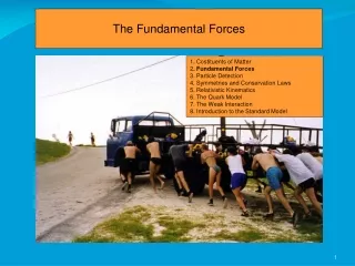
1. The Fundamental Forces 1. CostituentsofMatter 2. FundamentalForces 3. ParticleDetection 4. Symmetries and ConservationLaws 5. RelativisticKinematics 6. The Quark Model 7. The WeakInteraction 8. Introduction to the Standard Model

2. The concept of Force in classical and quantum physics • In Classical Physics : • Action at a distance • Field (Faraday, Maxwell) • Represented by force lines In Quantum Physics : • Exchange of Quanta Inverse square law In the case of classical fields the interaction is assumed to be instantaneous at a distance. However, this is not the case for Maxwell Theory (retarded potentials) or the Quantum Theories.

3. Classical and Quantum concepts of Force: (just) an analogy . . r Let us consider two particles at a separationdistance r If a source particle emits a quantum that reaches the other particle, the change in momentum will be: And since: We have: A concept of force based on the exchage of a force carrier. In a naive representation:

4. Fundamental Forces of Nature Gravity Strong Nuclear Force Weak Nuclear Force Guideline: explain all fundamental phenomena (phenomena between particles) with these interactions Electromagnetism

5. Electromagnetism Affects all particles with electric charge (Quarks, Leptons, W) Responsible of the bound between charged particles, e.g. atomic stability Coupling constant: the electric charge Range of the force: infinite Classical theory: Maxwell Equations (1861) F: Electromagnetic Field Tensor J: 4-current

6. Quantum Electrodynamics (QED) is the quantum relativistic theory of electromagnetic interactions. Its story begins with the Dirac Equation (1928) and goes on to its formulation as a gauge field theory as well as the study of its renormalizability (Bethe, Feynman, Tomonaga, Schwinger, Dyson 1956). F. Dyson showed the equivalence between the method of Feynman diagrams and the operatorial method of Tomonaga and Schwinger, making commonplace the use of Feynman diagrams for the description of fundamental interactions. A Feynman Diagram is a pictorial representation of a fundamental physical process that corresponds in a rigorous way to a mathematical expression. The pictorial representation is – however – more intuitive. The basic structure of the electromagnetic interaction (CGS): Fine structure constant It determines the intensity of the coupling at vertices of electromagnetic Feynman diagrams

7. Initial state Final state Propagator The Feynman Diagram and the (bosonic) Propagator: • Does not correspond to any physical process • If interpreted as a physical process, it would violate E-p conservation law • Two (or more) vertices diagrams have physical meaning time The concept of exchange of quanta (represented by the propagator) is the analog of the classical concept of a force field between two charges Interaction range estimate by using the static Klein-Gordon equation: Interaction strength (electric charge) Interaction range U(r) plays the role of scattering potential in configuration space, which can be analyzed in the (Fourier transformed) momentum space.

8. Classical and Quantum Fields Quantum Field: photons, creation and annihilation operators Classical Field: the role of quantum fluctuations is not important . The field can be described as a purely classical spacetime function. As an example, one can consider the scattering of electrons by an external e.m. field A, such as the field generated by an heavy nucleus. A static classical field would have the form: The scattering of an electron by the field of a heavy nucleus treated as a point charge is called Mott Scattering. Using the Coulomb gauge : The potential in space and momentum space are :

9. Propagator Potential Particle Momentum space Scattering amplitude for a particle in a potential Let us imagine a particle interacts with a coupling with a potential U Photon Propagator The propagator (scattering amplitude) associated to this potential : Momentum space Configuration space General scattering amplitude in a (boson-mediated) potential Propagator Couplings

10. (Scattering by a potential: the details) in this section

11. In the chosen system of units

12. Propagator Particle Particle Scattering amplitude and cross section Let us imagine the interaction of two Dirac (charged) particles Photon Propagator A typical matrix element for this process will have the form : And the Cross Section will have the form : Dirac Spinors Phase Space Flux Dirac currents

13. Feynman Diagrams Electrons in initial and final states time Intermediate virtual photon Scattering Rutherford Rutherford Scattering Well defined initial and final states The simplest Feynman Diagram given the initial and final states («tree level»). The diagram contains two vertices where the coupling constants appear. The diagram REPRESENTS the exchange of a virtual particle (the photon) between the charged particles that are the sources of the electromagnetic field. At every vertex, momentum and quantum numbers are conserved. Energy is not, as virtual (off-shell) particles are emitted or absorbed.

14. A taste of the S-Matrix expansion (and Feynman Diagrams) In a Theory of Interacting Quantum Fields Normal Product Fermion current interacting with the electromagnetic field Free Fermion field with mass m Free E.M. field The evolution of the system in the Interaction Picture is described by:

15. In a Scattering Process : Non-interacting particles in the initial state Non-interacting particles in the final state The solution of the general problem

16. Can be solved by iteration. Using : Where the series was cut at the second order. But one could continue like this : Power series expansion (Dyson Expansion) of the Scattering Matrix (power series in the Interaction Hamiltonian. Or power series in the interaction coupling constant

17. Feynman diagrams are a pictorial representation of this kind of perturbative series To every term of the series a diagram is associated following precise formal rules To every term in the S expansion a diagram can be drawn, following precise formal rules (outside of the goal of this course) + Fundamental (“tree level”) First order in Perturbation Theory While Feynman diagrams are NOT a picture of the real physical process (just a representation of a mathematical expression) they can give a lot of grasp on the physics at work. After all, Quantum Mechanics is just a representation!

18. Perturbation Theory: a few more ideas The occurrence probability of : It can by calculated by summing up the amplitudes due to various diagrams: 2 + …… = + + + Fundamental (“tree level”) First order in Perturbation Theory Higher-order terms in the expansion, which are negligible if the coupling constant is small. Which is the case of QED. The graphs have constituent lines (electrons) exchanging force carriers ( photons).

19. Bremsstrahlung Pair Production Lowest order of other electromagnetic processes :

20. Cross Section : (typical cross section of electromagnetic processes) Reaction rate Number of targets Incident flux Beam Attenuation : We assume no shadow effect between the targets in the slab (typical thin target approximation, area A, thickness Δx) Nuclear targets Incident flux Attenuation length

21. t Lifetimes and their relation to scattering processes Total amplitude Branching ratio of different final states Decay processes are represented by the same kind of diagrams that are used to describe scattering processes. The lifetime has a similar dependence on the coupling constants Electromagnetic processes: Partial amplitudes to different final states Beware the concept of “partial lifetime” (not an observable quantity) Lifetimes can be deduced from the characteristics of just one of the decay modes: Particle lifetime as a function of branching ratio and width of the i-th decay mode

22. Gravity Concerns all forms of energy of the Universe (mass included) Responsible of bounds between macroscopic bodies Classical field theory (Newton, 1687) for the masses Gravitational potential Mass density “Geometrized” spacetime field theory (Einstein, 1915) General Relativity The Principle of Equivalence between inertial mass (inertia to a force) and gravitational mass (gravitational charge) made it possible to consider gravity as a property of the spacetime background Far away from sources of mass/energy (in a flat spacetime) Einstein Tensor Cosmological Costant Energy-Momentum Tensor Metric Tensor

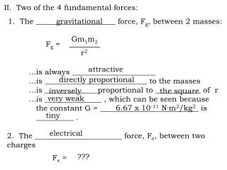
23. Gravity and Electromagnetism at the particle scale (the two classical theories) Same dependence on distance Fine structure constant Gravity constant (written in a way to show h and c) Now let us compare: Need to choose charges and masses. For the case of two protons ….gravity weaker by many orders of magnitude

24. Gravity is normally negligible at the atomic and subatomic level. But not at the Planck Mass: The Planck Mass can be defined as the mass that an elementary particle should have so that its gravitational interactions would be similar in strength to that of other interactions (electromagnetic,strong). Currently we have no valid quantum theory of gravity (in all regimes). If however such a theory exists, perhaps it could have a structure similar to QED: Electromagnetism Gravity GravitonSpin 2 PhotonSpin1 Charge Energy Two adimensional constants (at the mass and charge of the proton) Gravity Electromagnetism

25. The Planck scale The Schwarzschild Radius : the radius of a sphere such that, if all the mass of an object is compressed within that sphere, the escape speed from the surface of the sphere would equal the speed of light (wikipedia). Every massive object has a Schwarzschild radius : This neutron star is about to become a black hole Schwarzschild radius Generally a macroscopic bodies has dimensions much bigger than its Schwaszschild radius An object whose radius is smaller than the Schwarzschild radius is called a Black Hole Sun: Earth: Some notewhorty Schwarzschild radii :

26. Schwarzschild Black Hole (static and spherically symmetric) Sun: Earth: Smaller Black Holes have higher density What would be the density of the Sun as a Black Hole? Greater than the nuclear matter density ! But note that the mass is not uniformly distributed at r < rs

27. Flying away from the Schwarzschild Radius : A semiclassical calculation (does not replace a fully general-relativistc treatment) A Black Hole rs The kinetic energy of a massive body escaping from rs to infinity : The «classical» nonsense Incidentally gives the correct result for the Schwarzschild radius. Far away Nearby (but v<<c) Makes some sense (not much) WRONG !

28. The Compton Wavelength : instrinsic quantal space scale associated to a particle The concept of a Planck scale: 1. Schwarzschild Radius = Compton Wavelength The concept of a Planck scale: 2. Gravity on particles = Electromagnetism on particles (as shown before)

29. Can a high-energy heavy ion collider form a Black Hole? Heavy Ion Heavy Ion rs Even assuming that all the mass gets all the energy in a single elementary-like unit (which is utterly unrealistic because the collision happens at the level of the elementary constituents) Not enough mass to push the Compton wavelength below the Schwarzschild radius!

30. The three fundamental constants of the Universe Whatis the (only) way to form a length with theseconstants ? Whatis the (only) way to form a mass with theseconstants ? Whatis the (only) way to form a time with theseconstants ? One then has a Planck energy ..and a Planck temperature

31. The Planck scale in Astrophysics : How powerful can be an astrophysical object ? • Gamma Ray Bursts (energy emitted in e.m. form) • Active Galactic Nuclei (for a long time) • Supernovae for the first 100 s • Supernovae for the first month Planck Power : (Planck Energy) / (Planck Time) Absolute maximum of energy generation in a radius R Physical meaning : Mass entirely converted into energy in a time equal to the light crossing the gravitational radius of the object. Does not depend on microphysical scales.

32. Comparison between Gravitation and other Forces : Microscopic world (as before) : Compare with e.m: Need to choose charges and masses. The case of two protons: Macroscopic world : Let us consider, for instance, a little test mass on the surface of a compact massive object. What fraction ɛ of mc2 is the gravitational energy? M R m This defines the parameter ɛ (the same for any test mass, because of the Equivalence P) ɛ ~ 0.5 at the event horizon of a Schwarschild Black Hole (strong gravity regime) ɛ ~ 0.2 on the surface of a neutron star (still strong gravity regime) ɛ ~ 2 x 10-6 on the surface of the Sun

33. In General Relativity : actually: Energy (not just matter) A notewhorty application of General Relativity (with some assumptions regarding the matter distribution of the Universe) Cosmology The weak equivalence principle, also known as the universality of free fall or the Galilean equivalence principle can be stated in many ways. The strong EP includes (astronomic) bodies with gravitational binding energy (e.g., 1.74 solar-mass pulsar PSR J1903+0327, 15.3% of whose separated mass is absent as gravitational binding energy). The weak EP assumes falling bodies are bound by non-gravitational forces only. Either way, The trajectory of a point mass in a gravitational field depends only on its initial position and velocity, and is independent of its composition and structure.

34. Electromagnetic radiator • Two polarization states • Photon: spin 1 4-vector Graravitational radiator Flat spacetime curvature In the linearized (weak field) theory, far away from the source (in de Donder and Transverse Traceless gauge): • Four polarization states • Graviton: spin 2 Trace reverse h (tensor-like) • Electromagnetic waves discovered in 1886 (Hertz). • Gravitational waves observed in 2016

35. The Gravitational Multipole Expansion The potential generated by this mass distribution at x : Rewrite : The origin is the center of mass Intention : expand as a power series in r/x. Use trick: (Legendre poly for abs(x) and abs(z) less than one. Obtain : Dipole term goes to zero because of definition of the center of mass ! Obtain :

36. Gravity wave source candidates : • Systems whose mass distribution that changes rapidly in time. • High masses, small times. Black-holes, Neutron Stars merging. Supernovae. • Mass variation not having a spherical symmetry 1993 Hulse & Taylor measured the orbital decrease rate (7 mm/day) of the binary pulsar PSR B1913+16. This energy loss is in agreement with the prediction of General Relativity  indirect evidence for the emission of Gravitational Waves. Since (differently from electric charges) one has only one sign of the mass, the lowest moment is the 4-pole. Indirectevidence for gravitationalwaves

37. The search for Gravitational Waves: Michelson Interferometers in the Fabry-Pérot configuration Strain Sensitivity and location of Hanford and Livingston Interferometers (LIGO)

38. Detectors for gravitaty waves : Auriga, Nautilus, Explorer, LIGO, VIRGO… The VIRGO Interferometer (Cascina, Pisa) for the detection of gravitational waves

39. 14 September 2015: Hanford and Livingston observe at the same time (within 10 ms) a clear gravitational wave signal: GW150914, with full duration of 0.5 s. This kind of signal can be generated only by the mutual collapse of two Black-Holes having ~36 and 29 Solar Masses. The resulting (Kerr-type) Black Hole has 62 solar masses. Three solar masses have been transformed to energy (spacetime waves). Physical Review Letters 116 (2016) 061102. Raw Signals Background subtracted Background

40. The evidence in favor of a BH-BH scenario is compelling (only two BH’s can reach 75 Hz of mutual rotational frequency before merging in a region of Maximum power transformed into gravitational waves is about 1000 times a Supernova energy release! Spectacular confirmation of General Relativity as a classical theory.

41. Weak Nuclear Force Affects Quarks and Leptons (carriers of a “weak charge”) Generally, the Weak Nuclear process is dwarfed by Electromagnetic or Strong Nuclear processes. Weak Nuclear processes are commonplace whenever: • Conservation laws are violated (conserved in Strong or EM interactions) • Neutral particles and/or particles with no Strong Nuclear interaction intervene Neutron Beta Decay Let us get familiar with why some process just cannot take place Violates E conservation Violates conservation of baryon and lepton numbers Violates electric charge conservation The number of Baryons and Leptons cannot change arbitrarily:  Proton stability

42. “Specific” particles: • The Photon. Its presence is indicative of the Electromagnetic Interaction. • The Neutrino. This particle interacts only weakly. • W,Z. Appear only in Weak Interactions. Antineutrino absorption Are there Weak Interactions without neutrinos? Yes! It takes place through the Weak Interaction because it violates the Strangeness quantum number The decay diagram

43. 8B 8Be*+ e+ +e 2 The importance of Weak Interactions: the pp cycle in the Sun : 99,77% p + p  d+ e+ + e 0,23% p + e - + p d + e 84,7% d + p 3He + ~210-5 % 13,8% 3He + 4He 7Be +  13,78% 0,02% 7Be + e-7Li + e 7Be + p 8B +  3He+3He+2p 7Li + p ->+ 3He+p+e++e The pp cycle is responsible for ~98% of the energy generation in the Sun

44. An estimate of the Weak Coupling Constant (Weak) (Electromagnetic) Weak charge Weak Interaction Carriers and Propagator : W,Z mediating the interaction W± 80.4 GeV/c2 Spin 1 Z0 91.2 GeV/c2 Spin 1

45. Weak Interaction at low energies Let us consider again a Yukawa potential to describe the exchange of a carrier particle between matter fields (spin neglected) Static solutions : If MX=0  Poisson Eq for an electrostatic potential and for a charge –e interacting with a charge +e at the origin: justifying the definition of The general solution: If M  0, then R  ∞ that is again the e.m. style of interaction with coupling constants e,g If M is very large, then R 0 and the potential becomes very short range To gain the physical interpretation of this, let us go back to the amplitude

46. Probability amplitude for a particle to be scattered from initial to final momentum by the potential U Born approximation When M is big with respect to the momenta the scattering amplitude becomes a constant : When M is big with respect to the momenta the scattering amplitude becomes a constant : In the M∞ limit, Weak Interaction are characterized by g/MW :

47. The Range of the Weak Nuclear Interaction: 10-18 m Compton Wavelength argument : Weak Interactions Propagator : Low energies q2 << M2WZ The Fermi constant of the low energy Weak Interaction. An effective interaction of the form:

48. The Fermi Weak Coupling Constant It is often quoted as: What is actually meant is: Using the usual expression: One finds: As an example, the cross section for the process

49. Two fundamental types of Weak processes: • Charged Weak Currents: W exchange (a charged carrier W+ and W-) • Weak Neutral Currents: Z exchange (a neutral carrier, Z0) Photon-mediated Z-mediated W-mediated Z-mediated

50. Charged Currents Weak Interactions: Nuclear Beta Decay (at the nuclear level) (at the free neutron level) (at the fundamental constituents level) Charged Currents Weak Interactions: Antineutrino Scattering (at the free proton level) (at the fundamental constituents level) At the fundamental level, weak processes involve Quarks and Leptons (as well as weak carriers) :